Graphs of Linear Functions
We can now describe a variety of characteristics that explain the behavior of linear functions. We will use this information to analyze a graphed line and write an equation based on its observable properties. From evaluating the graph, what can you determine about this linear function?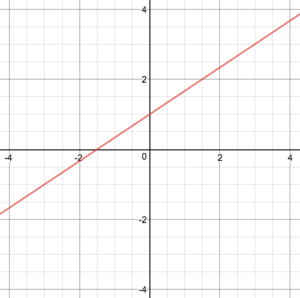 initial value (y-intercept)?
- one or two points?
- slope?
- increasing or decreasing?
- vertical or horizontal?
Graph Linear Functions
We previously saw that that the graph of a linear function is a straight line. We were also able to see the points of the function as well as the initial value from a graph. By graphing two functions, then, we can more easily compare their characteristics. There are three basic methods of graphing linear functions. The first is by plotting points and then drawing a line through the points. The second is by using the y-intercept and slope. And the third is by using transformations of the identity function [latex]f\left(x\right)=x[/latex].Graphing a Function by Plotting Points
To find points of a function, we can choose input values, evaluate the function at these input values, and calculate output values. The input values and corresponding output values form coordinate pairs. We then plot the coordinate pairs on a grid. In general, we should evaluate the function at a minimum of two inputs in order to find at least two points on the graph. For example, given the function, [latex]f\left(x\right)=2x[/latex], we might use the input values 1 and 2. Evaluating the function for an input value of 1 yields an output value of 2, which is represented by the point (1, 2). Evaluating the function for an input value of 2 yields an output value of 4, which is represented by the point (2, 4). Choosing three points is often advisable because if all three points do not fall on the same line, we know we made an error.How To: Given a linear function, graph by plotting points.
- Choose a minimum of two input values.
- Evaluate the function at each input value.
- Use the resulting output values to identify coordinate pairs.
- Plot the coordinate pairs on a grid.
- Draw a line through the points.
Example: Graphing by Plotting Points
Graph [latex]f\left(x\right)=-\frac{2}{3}x+5[/latex] by plotting points.Answer: Begin by choosing input values. This function includes a fraction with a denominator of 3, so let’s choose multiples of 3 as input values. We will choose 0, 3, and 6. Evaluate the function at each input value, and use the output value to identify coordinate pairs.
[latex]\begin{array}{l}x=0& & f\left(0\right)=-\frac{2}{3}\left(0\right)+5=5\Rightarrow \left(0,5\right)\\ x=3& & f\left(3\right)=-\frac{2}{3}\left(3\right)+5=3\Rightarrow \left(3,3\right)\\ x=6& & f\left(6\right)=-\frac{2}{3}\left(6\right)+5=1\Rightarrow \left(6,1\right)\end{array}[/latex]
Plot the coordinate pairs and draw a line through the points. The graph below is of the function [latex]f\left(x\right)=-\frac{2}{3}x+5[/latex].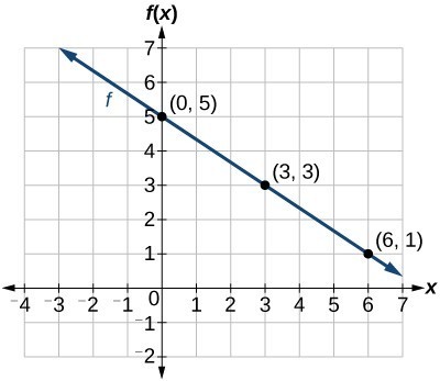
Analysis of the Solution
The graph of the function is a line as expected for a linear function. In addition, the graph has a downward slant, which indicates a negative slope. This is also expected from the negative constant rate of change in the equation for the function.Try It
Graph [latex]f\left(x\right)=-\frac{3}{4}x+6[/latex] by plotting points.Answer:

Graphing a Linear Function Using Transformations
Another option for graphing is to use transformations of the identity function [latex]f\left(x\right)=x[/latex]. A function may be transformed by a shift up, down, left, or right. A function may also be transformed using a reflection, stretch, or compression.Vertical Stretch or Compression
In the equation [latex]f\left(x\right)=mx[/latex], the m is acting as the vertical stretch or compression of the identity function. When m is negative, there is also a vertical reflection of the graph. Notice that multiplying the equation of [latex]f\left(x\right)=x[/latex] by m stretches the graph of f by a factor of m units if m > 1 and compresses the graph of f by a factor of m units if 0 < m < 1. This means the larger the absolute value of m, the steeper the slope.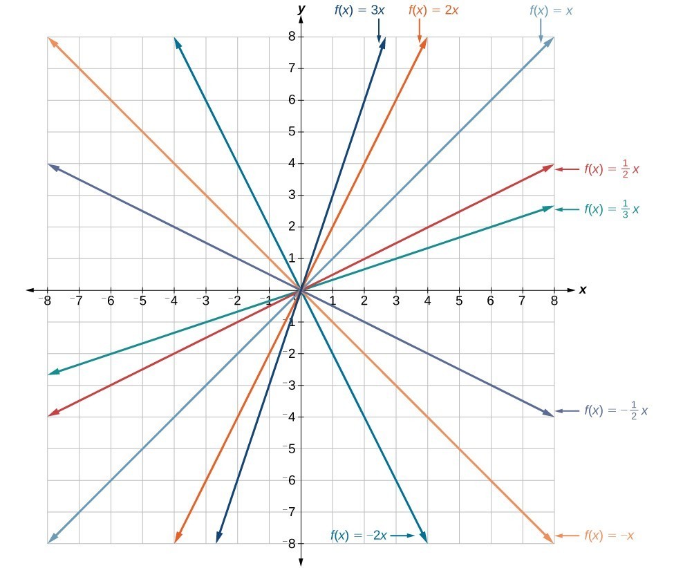 Vertical stretches and compressions and reflections on the function [latex]f\left(x\right)=x[/latex].
Vertical Shift
In [latex]f\left(x\right)=mx+b[/latex], the b acts as the vertical shift, moving the graph up and down without affecting the slope of the line. Notice that adding a value of b to the equation of [latex]f\left(x\right)=x[/latex] shifts the graph of f a total of b units up if b is positive and |b| units down if b is negative.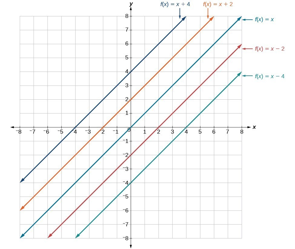 This graph illustrates vertical shifts of the function [latex]f\left(x\right)=x[/latex].
How To: Given the equation of a linear function, use transformations to graph the linear function in the form [latex]f\left(x\right)=mx+b[/latex].
- Graph [latex]f\left(x\right)=x[/latex].
- Vertically stretch or compress the graph by a factor m.
- Shift the graph up or down b units.
Example: Graphing by Using Transformations
Graph [latex]f\left(x\right)=\frac{1}{2}x - 3[/latex] using transformations.Answer: The equation for the function shows that [latex]m=\frac{1}{2}[/latex] so the identity function is vertically compressed by [latex]\frac{1}{2}[/latex]. The equation for the function also shows that [latex]b=-3[/latex] so the identity function is vertically shifted down 3 units. First, graph the identity function, and show the vertical compression.
 The function, [latex]y=x[/latex], compressed by a factor of [latex]\frac{1}{2}[/latex].
 The function [latex]y=\frac{1}{2}x[/latex], shifted down 3 units.
Try It
Graph [latex]f\left(x\right)=4+2x[/latex], using transformations.Answer: 
Q & A
In Example: Graphing by Using Transformations, could we have sketched the graph by reversing the order of the transformations? No. The order of the transformations follows the order of operations. When the function is evaluated at a given input, the corresponding output is calculated by following the order of operations. This is why we performed the compression first. For example, following the order: Let the input be 2.[latex]\begin{array}{l}f\text{(2)}=\frac{\text{1}}{\text{2}}\text{(2)}-\text{3}\hfill \\ =\text{1}-\text{3}\hfill \\ =-\text{2}\hfill \end{array}[/latex]
Write Equations of Linear Functions
We previously wrote the equation for a linear function from a graph. Now we can extend what we know about graphing linear functions to analyze graphs a little more closely. Begin by taking a look at the graph below. We can see right away that the graph crosses the y-axis at the point (0, 4) so this is the y-intercept.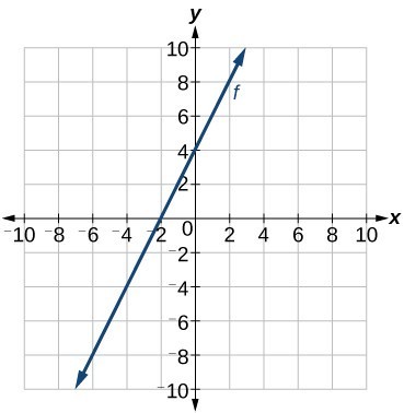 Then we can calculate the slope by finding the rise and run. We can choose any two points, but let’s look at the point (–2, 0). To get from this point to the y-intercept, we must move up 4 units (rise) and to the right 2 units (run). So the slope must be
[latex]m=\frac{\text{rise}}{\text{run}}=\frac{4}{2}=2[/latex]
Substituting the slope and y-intercept into the slope-intercept form of a line gives[latex]y=2x+4[/latex]
How To: Given a graph of linear function, find the equation to describe the function.
- Identify the y-intercept of an equation.
- Choose two points to determine the slope.
- Substitute the y-intercept and slope into the slope-intercept form of a line.
Example: Matching Linear Functions to Their Graphs
Match each equation of the linear functions with one of the lines in the graph below.- [latex]f\left(x\right)=2x+3[/latex]
- [latex]g\left(x\right)=2x - 3[/latex]
- [latex]h\left(x\right)=-2x+3[/latex]
- [latex]j\left(x\right)=\frac{1}{2}x+3[/latex]
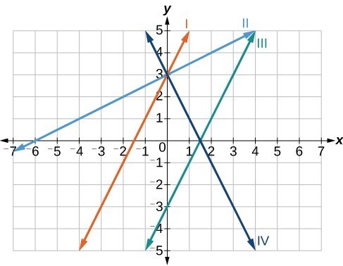
Answer: Analyze the information for each function.
- This function has a slope of 2 and a y-intercept of 3. It must pass through the point (0, 3) and slant upward from left to right. We can use two points to find the slope, or we can compare it with the other functions listed. Function g has the same slope, but a different y-intercept. Lines I and III have the same slant because they have the same slope. Line III does not pass through (0, 3) so f must be represented by line I.
- This function also has a slope of 2, but a y-intercept of –3. It must pass through the point (0, –3) and slant upward from left to right. It must be represented by line III.
- This function has a slope of –2 and a y-intercept of 3. This is the only function listed with a negative slope, so it must be represented by line IV because it slants downward from left to right.
- This function has a slope of [latex]\frac{1}{2}[/latex] and a y-intercept of 3. It must pass through the point (0, 3) and slant upward from left to right. Lines I and II pass through (0, 3), but the slope of j is less than the slope of f so the line for j must be flatter. This function is represented by Line II.

Finding the x-intercept of a Line
So far, we have been finding the y-intercepts of a function: the point at which the graph of the function crosses the y-axis. A function may also have an x-intercept, which is the x-coordinate of the point where the graph of the function crosses the x-axis. In other words, it is the input value when the output value is zero. To find the x-intercept, set a function f(x) equal to zero and solve for the value of x. For example, consider the function shown.[latex]f\left(x\right)=3x - 6[/latex]
Set the function equal to 0 and solve for x.[latex]\begin{array}{l}0=3x - 6\hfill \\ 6=3x\hfill \\ 2=x\hfill \\ x=2\hfill \end{array}[/latex]
The graph of the function crosses the x-axis at the point (2, 0).Q & A
Do all linear functions have x-intercepts? No. However, linear functions of the form y = c, where c is a nonzero real number are the only examples of linear functions with no x-intercept. For example, y = 5 is a horizontal line 5 units above the x-axis. This function has no x-intercepts.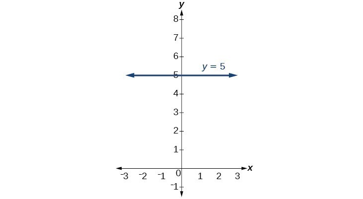
A General Note: x-intercept
The x-intercept of the function is value of x when f(x) = 0. It can be solved by the equation 0 = mx + b.Example: Finding an x-intercept
Find the x-intercept of [latex]f\left(x\right)=\frac{1}{2}x - 3[/latex].Answer: Set the function equal to zero to solve for x.
[latex]\begin{array}{l}0=\frac{1}{2}x - 3\\ 3=\frac{1}{2}x\\ 6=x\\ x=6\end{array}[/latex]
The graph crosses the x-axis at the point (6, 0).Analysis of the Solution
A graph of the function is shown below. We can see that the x-intercept is (6, 0) as we expected. The graph of the linear function [latex]f\left(x\right)=\frac{1}{2}x - 3[/latex].
Try It
Find the x-intercept of [latex]f\left(x\right)=\frac{1}{4}x - 4[/latex].Answer: [latex]\left(16,\text{ 0}\right)[/latex]
Example: Resistance of a Resistor
Electrical parts, such as resistors and capacitors, come with specified values of their operating parameters: resistance, capacitance, etc. However, due to imprecision in manufacturing, the actual values of these parameters vary somewhat from piece to piece, even when they are supposed to be the same. The best that manufacturers can do is to try to guarantee that the variations will stay within a specified range, often [latex]\pm 1\%,\pm5\%,[/latex] or [latex]\displaystyle\pm10\%[/latex]. Suppose we have a resistor rated at 680 ohms, [latex]\pm 5\%[/latex]. Use the absolute value function to express the range of possible values of the actual resistance.Answer: 5% of 680 ohms is 34 ohms. The absolute value of the difference between the actual and nominal resistance should not exceed the stated variability, so, with the resistance [latex]R[/latex] in ohms,
[latex]|R - 680|\le 34[/latex]
Try It
Students who score within 20 points of 80 will pass a test. Write this as a distance from 80 using absolute value notation.Answer: using the variable [latex]p[/latex] for passing, [latex]|p - 80|\le 20[/latex]
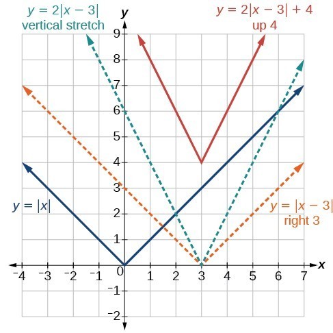
 The graph below is of [latex]y=2\left|x - 3\right|+4[/latex]. The graph of [latex]y=|x|[/latex] has been shifted right 3 units, vertically stretched by a factor of 2, and shifted up 4 units. This means that the corner point is located at [latex]\left(3,4\right)[/latex] for this transformed function.
Example: Writing an Equation for an Absolute Value Function
Write an equation for the function graphed below.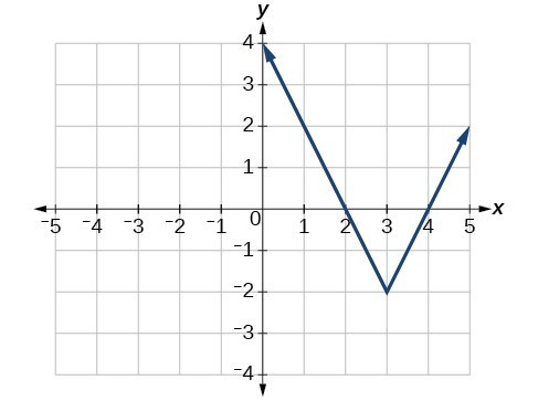
Answer:
The basic absolute value function changes direction at the origin, so this graph has been shifted to the right 3 units and down 2 units from the basic toolkit function.
 We also notice that the graph appears vertically stretched, because the width of the final graph on a horizontal line is not equal to 2 times the vertical distance from the corner to this line, as it would be for an unstretched absolute value function. Instead, the width is equal to 1 times the vertical distance.
 From this information we can write the equation
[latex]\begin{array}{l}f\left(x\right)=2\left|x - 3\right|-2,\hfill & \text{treating the stretch as a vertical stretch, or}\hfill \\ f\left(x\right)=\left|2\left(x - 3\right)\right|-2,\hfill & \text{treating the stretch as a horizontal compression}.\hfill \end{array}[/latex]
Analysis of the Solution
Note that these equations are algebraically equivalent—the stretch for an absolute value function can be written interchangeably as a vertical or horizontal stretch or compression.[latex]f\left(x\right)=a|x - 3|-2[/latex]
Now substituting in the point (1, 2)[latex]\begin{array}{l}2=a|1 - 3|-2\hfill \\ 4=2a\hfill \\ a=2\hfill \end{array}[/latex]
Try It
Write the equation for the absolute value function that is horizontally shifted left 2 units, is vertically flipped, and vertically shifted up 3 units.Answer: [latex]f\left(x\right)=-|x+2|+3\\[/latex]
Key Concepts
- Linear functions may be graphed by plotting points or by using the y-intercept and slope.
- Graphs of linear functions may be transformed by using shifts up, down, left, or right, as well as through stretches, compressions, and reflections.
- The y-intercept and slope of a line may be used to write the equation of a line.
- The x-intercept is the point at which the graph of a linear function crosses the x-axis.
- Horizontal lines are written in the form, [latex]f(x)=b[/latex].
- Vertical lines are written in the form, [latex]x=b[/latex].
- Parallel lines have the same slope.
- Perpendicular lines have negative reciprocal slopes, assuming neither is vertical.
- A line parallel to another line, passing through a given point, may be found by substituting the slope value of the line and the x- and y-values of the given point into the equation, [latex]f\left(x\right)=mx+b[/latex], and using the b that results. Similarly, the point-slope form of an equation can also be used.
- A line perpendicular to another line, passing through a given point, may be found in the same manner, with the exception of using the negative reciprocal slope.
- The absolute value function is commonly used to measure distances between points.
- Applied problems, such as ranges of possible values, can also be solved using the absolute value function.
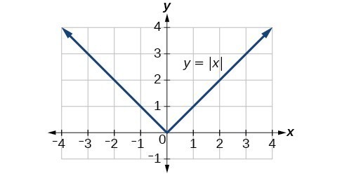
- The graph of the absolute value function resembles a letter V. It has a corner point at which the graph changes direction.
- In an absolute value equation, an unknown variable is the input of an absolute value function.
- If the absolute value of an expression is set equal to a positive number, expect two solutions for the unknown variable.
- An absolute value equation may have one solution, two solutions, or no solutions.
- An absolute value inequality is similar to an absolute value equation but takes the form [latex]|A|<B,|A|\le B,|A|>B,\text{ or }|A|\ge B[/latex]. It can be solved by determining the boundaries of the solution set and then testing which segments are in the set.
- Absolute value inequalities can also be solved graphically.
Glossary
absolute value equation an equation of the form [latex]|A|=B[/latex], with [latex]B\ge 0[/latex]; it will have solutions when [latex]A=B[/latex] or [latex]A=-B[/latex] absolute value inequality a relationship in the form [latex]|{ A }|<{ B },|{ A }|\le { B },|{ A }|>{ B },\text{or }|{ A }|\ge{ B }[/latex] horizontal line a line defined by [latex]f\left(x\right)=b[/latex], where b is a real number. The slope of a horizontal line is 0. parallel lines two or more lines with the same slope perpendicular lines two lines that intersect at right angles and have slopes that are negative reciprocals of each other vertical line a line defined by [latex]x=a[/latex], where a is a real number. The slope of a vertical line is undefined. x-intercept the point on the graph of a linear function when the output value is 0; the point at which the graph crosses the horizontal axisLicenses & Attributions
CC licensed content, Original
- Revision and Adaptation. Provided by: Lumen Learning License: CC BY: Attribution.
- Question ID 114584, 114587, 79757, 114592. Authored by: Lumen Learning. License: CC BY: Attribution. License terms: IMathAS Community License CC-BY + GPL.
CC licensed content, Shared previously
- College Algebra. Provided by: OpenStax Authored by: Abramson, Jay et al.. Located at: https://openstax.org/books/college-algebra/pages/1-introduction-to-prerequisites. License: CC BY: Attribution. License terms: Download for free at http://cnx.org/contents/[email protected].
- Question ID 69981. Authored by: Majerus, Ryan. License: CC BY: Attribution. License terms: IMathAS Community License CC-BY + GPL.
- Question ID 88183. Authored by: Shahbazian, Roy. License: CC BY: Attribution. License terms: IMathAS Community License CC-BY + GPL.
- Precalculus. Provided by: OpenStax Authored by: Jay Abramson, et al.. License: CC BY: Attribution. License terms: Download For Free at : http://cnx.org/contents/[email protected]..
- Question ID 1440. Authored by: unknown, mb Lippman,David. License: CC BY: Attribution. License terms: IMathAS Community License CC-BY + GPL.
- Question ID 15599. Authored by: Johns, Bryan . License: CC BY: Attribution. License terms: IMathAS Community License CC-BY + GPL.
- Question ID 469. Authored by: WebWork-Rochester, mb Lippman, David. License: CC BY: Attribution. License terms: IMathAS Community License CC-BY + GPL.
- Question ID 60791. Authored by: Day, Alyson. License: CC BY: Attribution. License terms: IMathAS Community License CC-BY + GPL.
- Question ID 40657. Authored by: Michael Jenck. License: CC BY: Attribution. License terms: IMathAS Community License CC-BY + GPL.
