Partial Derivatives
Functions of Several Variables
Multivariable calculus is the extension of calculus in one variable to calculus in more than one variable.Learning Objectives
Identify areas of application of multivariable calculusKey Takeaways
Key Points
- Multivariable calculus can be applied to analyze deterministic systems that have multiple degrees of freedom.
- Unlike a single variable function [latex]f(x)[/latex], for which the limits and continuity of the function need to be checked as [latex]x[/latex] varies on a line ([latex]x[/latex]-axis), multivariable functions have infinite number of paths approaching a single point.
- In multivariable calculus, gradient, Stokes', divergence, and Green theorems are specific incarnations of a more general theorem: the generalized Stokes' theorem.
Key Terms
- deterministic: having exactly predictable time evolution
- divergence: a vector operator that measures the magnitude of a vector field's source or sink at a given point, in terms of a signed scalar
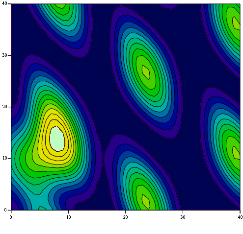
A Scalar Field: A scalar field shown as a function of [latex](x,y)[/latex]. Extensions of concepts used for single variable functions may require caution.
Limits and Continuity
A study of limits and continuity in multivariable calculus yields counter-intuitive results not demonstrated by single-variable functions.Learning Objectives
Describe the relationship between the multivariate continuity and the continuity in each argumentKey Takeaways
Key Points
- The function [latex]f(x,y) = \frac{x^2y}{x^4+y^2}[/latex] has different limit values at the origin, depending on the path taken for the evaluation.
- Continuity in each argument does not imply multivariate continuity.
- When taking different paths toward the same point yields different values for the limit, the limit does not exist.
Key Terms
- continuity: lack of interruption or disconnection; the quality of being continuous in space or time
- limit: a value to which a sequence or function converges
- scalar function: any function whose domain is a vector space and whose value is its scalar field
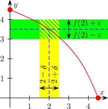
Continuity: Continuity in single-variable function as shown is rather obvious. However, continuity in multivariable functions yields many counter-intuitive results.
Partial Derivatives
A partial derivative of a function of several variables is its derivative with respect to a single variable, with the others held constant.Learning Objectives
Identify proper ways to express the partial derivativeKey Takeaways
Key Points
- The partial derivative of a function [latex]f[/latex] with respect to the variable [latex]x[/latex] is variously denoted by [latex]f^\prime_x,\ f_{,x},\ \partial_x f, \text{ or } \frac{\partial f}{\partial x}[/latex].
- To every point on this surface describing a multi-variable function, there is an infinite number of tangent lines. Partial differentiation is the act of choosing one of these lines and finding its slope.
- As an ordinary derivative, partial derivatives are defined in limit: [latex]\frac{ \partial }{\partial a_i }f(\mathbf{a}) = \lim_{h \rightarrow 0}{ f(a_1, \dots, a_{i-1}, a_i+h, a_{i+1}, \dots,a_n) - f(a_1, \dots, a_i, \dots,a_n) \over h }[/latex].
Key Terms
- differential geometry: the study of geometry using differential calculus
- Euclidean: adhering to the principles of traditional geometry, in which parallel lines are equidistant
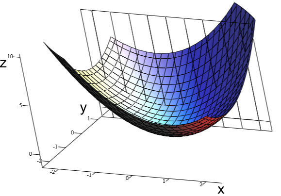
Graph of [latex]z = x^2 + xy + y^2[/latex]: For the partial derivative at [latex](1, 1, 3)[/latex] that leaves [latex]y[/latex] constant, the corresponding tangent line is parallel to the [latex]xz[/latex]-plane.
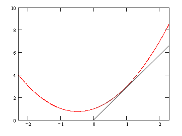
Graph of [latex]z = x^2 + xy + y^2[/latex] at [latex]y=1[/latex]: A slice of the graph at [latex]y=1[/latex].
Formal Definition
Like ordinary derivatives, the partial derivative is defined as a limit. Let [latex]U[/latex] be an open subset of [latex]R^n[/latex] and [latex]f:U \rightarrow R[/latex] a function. The partial derivative of [latex]f[/latex] at the point [latex]a = (a_1, \cdots, a_n) \in U[/latex] with respect to the [latex]i[/latex]th variable is defined as: [latex-display]\displaystyle{\frac{ \partial }{\partial a_i }f(\mathbf{a}) = \lim_{h \rightarrow 0}{ f(a_1, \cdots, a_{i-1}, a_i+h, a_{i+1}, \cdots,a_n) - f(a_1, \cdots, a_i, \cdots,a_n) \over h }}[/latex-display]Tangent Planes and Linear Approximations
The tangent plane to a surface at a given point is the plane that "just touches" the surface at that point.Learning Objectives
Explain why the tangent plane can be used to approximate the surface near the pointKey Takeaways
Key Points
- For a surface given by a differentiable multivariable function [latex]z=f(x,y)[/latex], the equation of the tangent plane at [latex](x_0,y_0,z_0)[/latex] is given as fx(x0,y0)(x−x0)+fy(x0,y0)(y−y0)−(z−z0)=0f_x(x_0,y_0) (x-x_0) + f_y(x_0,y_0) (y-y_0) - (z-z_0) = 0.
- Since a tangent plane is the best approximation of the surface near the point where the two meet, the tangent plane can be used to approximate the surface near the point.
- The plane describing the linear approximation for a surface described by [latex]z=f(x,y)[/latex] is given as [latex]z = z_0 + f_x(x_0,y_0) (x-x_0) + f_y(x_0,y_0) (y-y_0)[/latex].
Key Terms
- differentiable: having a derivative, said of a function whose domain and co-domain are manifolds
- differential geometry: the study of geometry using differential calculus
- slope: also called gradient; slope or gradient of a line describes its steepness

Tangent Plane to a Sphere: The tangent plane to a surface at a given point is the plane that "just touches" the surface at that point.
Equations
When the curve is given by [latex]y = f(x)[/latex] the slope of the tangent is [latex]\frac{dy}{dx}[/latex], so by the point–slope formula the equation of the tangent line at [latex](x_0, y_0)[/latex] is: [latex-display]\frac{dy}{dx}(x_0,y_0) \cdot (x-x_0) - (y-y_0)[/latex-display] where [latex](x, y)[/latex] are the coordinates of any point on the tangent line, and where the derivative is evaluated at [latex]x=x_0[/latex]. The tangent plane to a surface at a given point [latex]p[/latex] is defined in an analogous way to the tangent line in the case of curves. It is the best approximation of the surface by a plane at [latex]p[/latex], and can be obtained as the limiting position of the planes passing through 3 distinct points on the surface close to [latex]p[/latex] as these points converge to [latex]p[/latex]. For a surface given by a differentiable multivariable function [latex]z=f(x,y)[/latex], the equation of the tangent plane at [latex](x_0,y_0,z_0)[/latex] is given as: [latex-display]f_x(x_0,y_0) (x-x_0) + f_y(x_0,y_0) (y-y_0) - (z-z_0) = 0[/latex-display] where [latex](x_0,y_0,z_0)[/latex] is a point on the surface. Note the similarity of the equations for tangent line and tangent plane.Linear Approximation
Since a tangent plane is the best approximation of the surface near the point where the two meet, tangent plane can be used to approximate the surface near the point. The approximation works well as long as the point [latex](x,y,z) [/latex] under consideration is close enough to [latex](x_0,y_0,z_0)[/latex], where the tangent plane touches the surface. The plane describing the linear approximation for a surface described by [latex]z=f(x,y)[/latex] is given as: [latex]z = z_0 + f_x(x_0,y_0) (x-x_0) + f_y(x_0,y_0) (y-y_0)[/latex].The Chain Rule
For a function [latex]U[/latex] with two variables [latex]x[/latex] and [latex]y[/latex], the chain rule is given as [latex]\frac{d U}{dt} = \frac{\partial U}{\partial x} \cdot \frac{dx}{dt} + \frac{\partial U}{\partial y} \cdot \frac{dy}{dt}[/latex].Learning Objectives
Express a chain rule for a function with two variablesKey Takeaways
Key Points
- The chain rule can be easily generalized to functions with more than two variables.
- For a single variable functions, the chain rule is a formula for computing the derivative of the composition of two or more functions. For example, the chain rule for [latex]f \circ g (x) ≡ f [g (x)][/latex] is [latex]\frac {df}{dx} = \frac {df}{dg} \cdot \frac {dg}{dx}[/latex].
- The chain rule can be used when we want to calculate the rate of change of the function [latex]U(x,y)[/latex] as a function of time [latex]t[/latex], where [latex]x=x(t)[/latex] and [latex]y=y(t)[/latex].
Key Terms
- potential energy: the energy possessed by an object because of its position (in a gravitational or electric field), or its condition (as a stretched or compressed spring, as a chemical reactant, or by having rest mass)
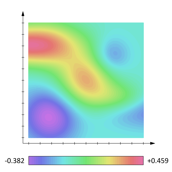
Scalar Field: The chain rule can be used to take derivatives of multivariable functions with respect to a parameter.
Example
For [latex]z = (x^2 + xy + y^2)^{1/2}[/latex] where [latex]x=x(t)[/latex] and [latex]y=y(t)[/latex], express [latex]\frac{dz}{dt}[/latex] in terms of [latex]\frac{dx}{dt}[/latex]and [latex]\frac{dy}{dt}[/latex]: [latex-display]\displaystyle{\frac{dz}{dt} = \frac{d}{dt}(x^2 +xy+ y^2)^{1/2}}[/latex-display] [latex-display]\displaystyle{\,\,\,\quad= \frac{1}{2}(x^2 +xy + y^2)^{-1/2}\frac{d}{dt}(x^2 +xy+ y^2)}[/latex-display] [latex-display]\displaystyle{\,\,\,\quad=\frac{1}{2}(x^2 +xy+ y^2)^{-1/2}\left(\frac{d}{dt}(x^2) + \frac{d}{dt}(xy) +\frac{d}{dt}(y^2) \right)}[/latex-display] [latex-display]\displaystyle{\,\,\,\quad= \frac{ \left(x+\displaystyle{\frac{1}{2}} y \right)\displaystyle{\frac{dx}{dt}} + \left(y+\frac{1}{2} x \right) \displaystyle{\frac{dy}{dt}}}{\sqrt{x^2 +xy+ y^2}}}[/latex-display]Directional Derivatives and the Gradient Vector
The directional derivative represents the instantaneous rate of change of the function, moving through [latex]\mathbf{x}[/latex] with a velocity specified by [latex]\mathbf{v}[/latex].Learning Objectives
Describe properties of a function represented by the directional derivativeKey Takeaways
Key Points
- The directional derivative is defined by the limit [latex]\nabla_{\mathbf{v}}{f}(\mathbf{x}) = \lim_{h \rightarrow 0}{\frac{f(\mathbf{x} + h\mathbf{v}) - f(\mathbf{x})}{h}}[/latex].
- If the function [latex]f[/latex] is differentiable at [latex]\mathbf{x}[/latex], then the directional derivative exists along any vector [latex]\mathbf{v}[/latex], and one gets [latex]\nabla_{\mathbf{v}}{f}(\mathbf{x}) = \nabla f(\mathbf{x}) \cdot \mathbf{v}[/latex].
- Many of the familiar properties of the ordinary derivative hold for the directional derivative.
Key Terms
- chain rule: a formula for computing the derivative of the composition of two or more functions.
- gradient: of a function [latex]y=f(x)[/latex] or the graph of such a function, the rate of change of [latex]y[/latex] with respect to [latex]x[/latex]; that is, the amount by which [latex]y[/latex] changes for a certain (often unit) change in [latex]x[/latex].
Definition
The directional derivative of a scalar function [latex]f(\mathbf{x}) = f(x_1, x_2, \ldots, x_n)[/latex] along a vector [latex]\mathbf{v} = (v_1, \ldots, v_n)[/latex] is the function defined by the limit: [latex-display]\displaystyle{\nabla_{\mathbf{v}}{f}(\mathbf{x}) = \lim_{h \rightarrow 0}{\frac{f(\mathbf{x} + h\mathbf{v}) - f(\mathbf{x})}{h}}}[/latex-display] If the function [latex]f[/latex] is differentiable at [latex]\mathbf x[/latex], then the directional derivative exists along any vector [latex]\mathbf v[/latex], and one has [latex]\nabla_{\mathbf{v}}{f}(\mathbf{x}) = \nabla f(\mathbf{x}) \cdot \mathbf{v}[/latex], where the [latex]\nabla f(\mathbf{x})[/latex] is the gradient vector and [latex]\cdot[/latex] is the dot product. At any point [latex]\mathbf x[/latex], the directional derivative of [latex]f[/latex] intuitively represents the rate of change of [latex]f[/latex] with respect to time when it is moving at a speed and direction given by [latex]\mathbf v[/latex] at the point [latex]\mathbf x[/latex]. The name "directional derivative" is a bit misleading since it depends on both the length and direction of [latex]\mathbf v[/latex]. We can imagine the directional derivative [latex]\nabla_{\mathbf{v}}{f}(\mathbf{x})[/latex] as the slope of the tangent line to the 2-dimensional slice of the graph of [latex]f[/latex] that lies parallel to the vector [latex]\mathbf{v}[/latex]. However, this slice will be stretched or compressed horizontally unless [latex]\mathbf{v}=1[/latex].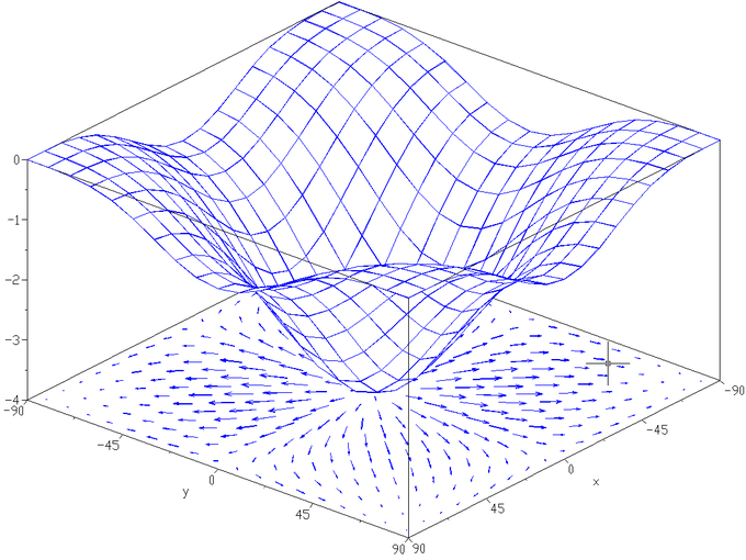
Gradient of a Function: The gradient of the function [latex]f(x,y) = −\left((\cos x)^2 + (\cos y)^2\right)[/latex] depicted as a projected vector field on the bottom plane. Directional derivative represents the rate of change of the function along any direction specified by [latex]\mathbf{v}[/latex].
Properties
Many of the familiar properties of the ordinary derivative hold for the directional derivative.The Sum Rule
[latex-display]\nabla_\mathbf{v} (f + g) = \nabla_\mathbf{v} f + \nabla_\mathbf{v} g[/latex-display]The Constant Factor Rule
For any constant [latex]c[/latex], [latex]\nabla_\mathbf{v} (cf) = c\nabla_\mathbf{v} f[/latex].The Product Rule (or Leibniz Rule)
[latex-display]\nabla_\mathbf{v} (fg) = g\nabla_\mathbf{v} f + f\nabla_\mathbf{v} g[/latex-display]The Chain Rule
If [latex]g[/latex] is differentiable at [latex]p[/latex] and [latex]h[/latex] is differentiable at [latex]g(p)[/latex], then [latex]\nabla_\mathbf{v} h\circ g (p) = h'(g(p)) \nabla_\mathbf{v} g (p)[/latex].Maximum and Minimum Values
The second partial derivative test is a method used to determine whether a critical point is a local minimum, maximum, or saddle point.Learning Objectives
Apply the second partial derivative test to determine whether a critical point is a local minimum, maximum, or saddle pointKey Takeaways
Key Points
- For a function of two variables, the second partial derivative test is based on the sign of [latex]M(x,y)= f_{xx}(x,y)f_{yy}(x,y) - \left( f_{xy}(x,y) \right)^2[/latex] and [latex]f_{xx}(a,b)[/latex], where [latex](a,b)[/latex] is a critical point.
- There are substantial differences between the functions of one variable and the functions of more than one variable in the identification of global extrema.
- The maximum and minimum of a function, known collectively as extrema, are the largest and smallest values that the function takes at a point either within a given neighborhood (local or relative extremum) or on the function domain in its entirety (global or absolute extremum).
Key Terms
- critical point: a maximum, minimum, or point of inflection on a curve; a point at which the derivative of a function is zero or undefined
- intermediate value theorem: a statement that claims that, for each value between the least upper bound and greatest lower bound of the image of a continuous function, there is a corresponding point in its domain that the function maps to that value
- Rolle's theorem: a theorem stating that a differentiable function which attains equal values at two distinct points must have a point somewhere between them where the first derivative (the slope of the tangent line to the graph of the function) is zero
Finding Maxima and Minima of Multivariable Functions
The second partial derivative test is a method in multivariable calculus used to determine whether a critical point [latex](a,b, \cdots )[/latex] of a function [latex]f(x,y, \cdots )[/latex] is a local minimum, maximum, or saddle point.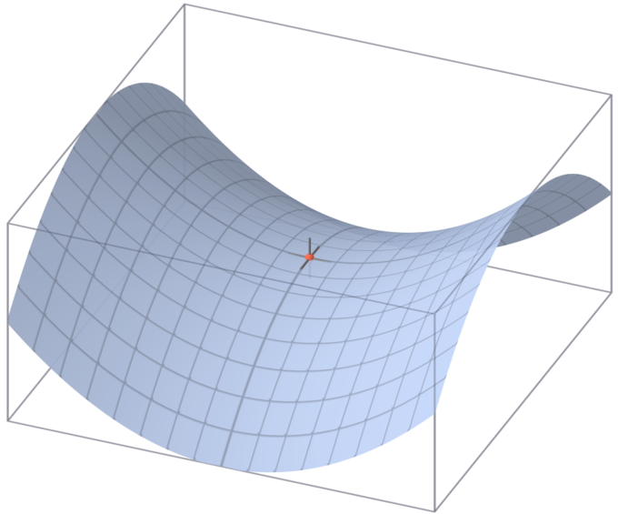
Saddle Point: A saddle point on the graph of [latex]z=x^2−y^2[/latex] (in red).
- If [latex]M(a,b)>0[/latex] and [latex]f_{xx}(a,b)>0[/latex], then [latex](a,b)[/latex] is a local minimum of [latex]f[/latex].
- If M(a,b)>0M(a,b)>0 and fxx(a,b)<0f_{xx}(a,b)<0, then [latex](a,b)[/latex] is a local maximum of [latex]f[/latex].
- If [latex]M(a,b)<0[/latex], then [latex](a,b)[/latex] is a saddle point of [latex]f[/latex].
- If [latex]M(a,b)=0[/latex], then the second derivative test is inconclusive.
Lagrange Multiplers
The method of Lagrange multipliers is a strategy for finding the local maxima and minima of a function subject to equality constraints.Learning Objectives
Describe application of the method of Lagrange multipliersKey Takeaways
Key Points
- To maximize [latex]f(x,y)[/latex] subject to [latex]g(x,y)=c[/latex], we introduce a new variable [latex]\lambda[/latex], called a Lagrange multiplier, and study the Lagrange function (or Lagrangian) defined by [latex]\Lambda(x,y,\lambda) = f(x,y) + \lambda \cdot \Big(g(x,y)-c\Big)[/latex].
- When the contour line for [latex]g = c[/latex] meets the contour lines of [latex]f[/latex] tangentially do we not increase or decrease the value of [latex]f[/latex] — that is, when the contour lines touch but do not cross. This will often be the situation where a solution to the constrained maximum problem above exists.
- Solve [latex]\nabla_{x,y,\lambda} \Lambda(x, y, \lambda)=0[/latex], and we find a necessary condition for extrema under the given constraint.
Key Terms
- gradient: of a function [latex]y = f(x)[/latex] or the graph of such a function, the rate of change of [latex]y[/latex] with respect to [latex]x[/latex]; that is, the amount by which [latex]y[/latex] changes for a certain (often unit) change in [latex]x[/latex]
- contour: a line on a map or chart delineating those points which have the same altitude or other plotted quantity: a contour line or isopleth
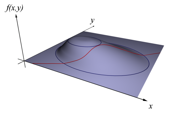
Maximizing f(x,y): Find x and y to maximize f(x,y) subject to a constraint (shown in red) g(x,y)=c.
Introduction
One of the most common problems in calculus is that of finding maxima or minima (in general, "extrema") of a function, but it is often difficult to find a closed form for the function being extremized. Such difficulties often arise when one wishes to maximize or minimize a function subject to fixed outside conditions or constraints. The method of Lagrange multipliers is a powerful tool for solving this class of problems without the need to explicitly solve the conditions and use them to eliminate extra variables. Consider the two-dimensional problem introduced above. Maximize [latex]f(x,y)[/latex] subject to [latex]g(x,y)=c[/latex]. We can visualize contours of [latex]f[/latex] given by [latex]f(x, y)=d[/latex] for various values of [latex]d[/latex], and the contour of [latex]g[/latex] given by [latex]g (x, y) = c[/latex]. Suppose we walk along the contour line with [latex]g = c[/latex]. In general, the contour lines of [latex]f[/latex] and [latex]g[/latex] may be distinct, so following the contour line for [latex]g = c[/latex], one could intersect with or cross the contour lines of [latex]f[/latex]. This is equivalent to saying that while moving along the contour line for [latex]g = c[/latex], the value of [latex]f[/latex] can vary. When the contour line for [latex]g = c[/latex] meets contour lines of [latex]f[/latex] tangentially we neither increase nor decrease the value of [latex]f[/latex]—that is, when the contour lines touch but do not cross. The contour lines of [latex]f[/latex] and [latex]g[/latex] touch when the tangent vectors of the contour lines are parallel. Since the gradient of a function is perpendicular to the contour lines, this is the same as saying that the gradients of [latex]f[/latex] and [latex]g[/latex] are parallel. Thus, we want points: [latex-display](x,y)[/latex] where [latex]g(x,y)=c[/latex-display] and [latex]\nabla_{x,y} f = - \lambda \nabla_{x,y} g[/latex], where [latex]\nabla_{x,y} f= \left( \frac{\partial f}{\partial x}, \frac{\partial f}{\partial y} \right)[/latex] and [latex]\nabla_{x,y} g= \left( \frac{\partial g}{\partial x}, \frac{\partial g}{\partial y} \right)[/latex] are the respective gradients. The constant is required because, although the two gradient vectors are parallel, the magnitudes of the gradient vectors are generally not equal. Note that [latex]\lambda \neq 0[/latex]; otherwise we cannot assert the two gradients are parallel. To incorporate these conditions into one equation, we introduce an auxiliary function, [latex]\Lambda(x,y,\lambda) = f(x,y) + \lambda \cdot \Big(g(x,y)-c\Big)[/latex], and solve [latex]\nabla_{x,y,\lambda} \Lambda(x, y, \lambda)=0[/latex]. This is the method of Lagrange multipliers. Note that [latex]\nabla_{\lambda} \Lambda(x, y, \lambda)=0[/latex] implies [latex]g(x,y)=c[/latex]. Where the Lagrange multiplier [latex]\lambda=0[/latex] we can have a local extremum and the two contours cross instead of meeting tangentially. Consider the following example. Minimize [latex]f(x,y) = \sin(x)[/latex], given that [latex]g(x,y) = x^2 + y^2=9[/latex]. Every point [latex]\left(\frac{-\pi}{2}, y\right)[/latex][latex]f=-1[/latex] is a global minimum of [latex]f[/latex] with value [latex]-1[/latex]. Therefore where the constraint [latex]g=c[/latex] crosses the contour line [latex]f=-1[/latex], is a local minimum of [latex]f[/latex] on the constraint. The trace and the contour [latex]f=-1[/latex] cross at the minimum as we can see in the figure. It is easy to verify that [latex]f_x=0[/latex] and [latex]f_y=0[/latex] when [latex]x = \frac{\pi}{2}[/latex]. Since both [latex]g_x \neq 0[/latex] and [latex]g_y \neq 0[/latex], the Lagrange multiplier [latex]\lambda = 0[/latex] at the minimum.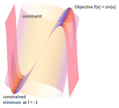
Example where the contour and constraint cross at an extremum.
Optimization in Several Variables
To solve an optimization problem, formulate the function [latex]f(x,y, \cdots )[/latex] to be optimized and find all critical points first.Learning Objectives
Solve a simple problem that requires optimization of several variablesKey Takeaways
Key Points
- Mathematical optimization is the selection of a best element (with regard to some criteria) from some set of available alternatives.
- An optimization process that involves only a single variable is rather straightforward. After finding out the function [latex]f(x)[/latex] to be optimized, local maxima or minima at critical points can easily be found. End points may have maximum/minimum values as well.
- For a rectangular cuboid shape, given the fixed volume, a cube is the geometric shape that minimizes the surface area.
Key Terms
- optimization: the design and operation of a system or process to make it as good as possible in some defined sense
- cuboid: a parallelepiped having six rectangular faces
Cardboard Box with a Fixed Volume
A packaging company needs cardboard boxes in rectangular cuboid shape with a given volume of 1000 cubic centimeters and would like to minimize the material cost for the boxes. What should be the dimensions [latex]x[/latex], [latex]y[/latex], [latex]z[/latex] of a box? First of all, the material cost would be proportional to the surface area [latex]S[/latex] of the cuboid. Therefore, the goal of the optimization is to minimize a function [latex]S(x,y,z) = 2(xy + yz+zx)[/latex]. The constraint in the case is that the volume is fixed: [latex]V = xyz = 1000[/latex].
Rectangular Cuboid: Mathematical optimization can be used to solve problems that involve finding the right size of a volume such as a cuboid.
Applications of Minima and Maxima in Functions of Two Variables
Finding extrema can be a challenge with regard to multivariable functions, requiring careful calculation.Learning Objectives
Identify steps necessary to find the minimum and maximum in multivariable functionsKey Takeaways
Key Points
- The second derivative test is a criterion for determining whether a given critical point of a real function of one variable is a local maximum or a local minimum using the value of the second derivative at the point.
- To find minima/maxima for functions with two variables, we must first find the first partial derivatives with respect to [latex]x[/latex] and [latex]y[/latex] of the function.
- The function [latex]z = f(x, y) = (x+y)(xy + xy^2)[/latex] has saddle points at [latex](0,-1)[/latex] and [latex](1,-1)[/latex] and a local maximum at [latex]\left(\frac{3}{8}, -3.4\right)[/latex].
Key Terms
- multivariable: concerning more than one variable
- critical point: a maximum, minimum, or point of inflection on a curve; a point at which the derivative of a function is zero or undefined
Example
Find and label the critical points of the following function: [latex-display]z = f(x, y) = (x+y)(xy + xy^2)[/latex-display]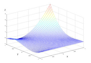 Plot of [latex]z = (x+y)(xy+xy^2)[/latex]: The maxima and minima of this plot cannot be found without extensive calculation.
- [latex]D(0, 0) = 0[/latex]
- [latex]D(0, -1) = -1[/latex]
- [latex]D(1, -1) = -1[/latex]
- [latex]D\left(\frac{3}{8}, -\frac{3}{4}\right) = 0.210938[/latex]
- at (0, −1), [latex]f(x, y)[/latex] has a saddle point
- at (1, −1), [latex]f(x, y)[/latex] has a saddle point
- at [latex]\left(\frac{3}{8}, -\frac{3}{4}\right)[/latex] [latex]f(x, y)[/latex] has a local maximum, since [latex]f_{xx} = -\frac{3}{8} < 0[/latex]
Licenses & Attributions
CC licensed content, Shared previously
- Curation and Revision. Provided by: Boundless.com License: CC BY-SA: Attribution-ShareAlike.
CC licensed content, Specific attribution
- Multivariable calculus. Provided by: Wikipedia License: CC BY-SA: Attribution-ShareAlike.
- deterministic. Provided by: Wiktionary License: CC BY-SA: Attribution-ShareAlike.
- divergence. Provided by: Wiktionary License: CC BY-SA: Attribution-ShareAlike.
- Multivariable calculus. Provided by: Wikipedia License: CC BY: Attribution.
- Multivariable calculus. Provided by: Wikipedia License: CC BY-SA: Attribution-ShareAlike.
- continuity. Provided by: Wiktionary License: CC BY-SA: Attribution-ShareAlike.
- limit. Provided by: Wiktionary License: CC BY-SA: Attribution-ShareAlike.
- scalar function. Provided by: Wiktionary License: CC BY-SA: Attribution-ShareAlike.
- Multivariable calculus. Provided by: Wikipedia License: CC BY: Attribution.
- Continuous function. Provided by: Wikipedia License: CC BY: Attribution.
- Partial derivative. Provided by: Wikipedia License: CC BY-SA: Attribution-ShareAlike.
- Euclidean. Provided by: Wiktionary License: CC BY-SA: Attribution-ShareAlike.
- differential geometry. Provided by: Wiktionary License: CC BY-SA: Attribution-ShareAlike.
- Multivariable calculus. Provided by: Wikipedia License: CC BY: Attribution.
- Continuous function. Provided by: Wikipedia License: CC BY: Attribution.
- Partial derivative. Provided by: Wikipedia License: CC BY: Attribution.
- Partial derivative. Provided by: Wikipedia License: CC BY: Attribution.
- Tangent. Provided by: Wikipedia License: CC BY-SA: Attribution-ShareAlike.
- differentiable. Provided by: Wiktionary License: CC BY-SA: Attribution-ShareAlike.
- slope. Provided by: Wiktionary License: CC BY-SA: Attribution-ShareAlike.
- differential geometry. Provided by: Wiktionary License: CC BY-SA: Attribution-ShareAlike.
- Multivariable calculus. Provided by: Wikipedia License: CC BY: Attribution.
- Continuous function. Provided by: Wikipedia License: CC BY: Attribution.
- Partial derivative. Provided by: Wikipedia License: CC BY: Attribution.
- Partial derivative. Provided by: Wikipedia License: CC BY: Attribution.
- Tangent. Provided by: Wikipedia License: CC BY: Attribution.
- Chain rule. Provided by: Wikipedia License: CC BY-SA: Attribution-ShareAlike.
- potential energy. Provided by: Wikipedia License: CC BY-SA: Attribution-ShareAlike.
- Multivariable calculus. Provided by: Wikipedia License: CC BY: Attribution.
- Continuous function. Provided by: Wikipedia License: CC BY: Attribution.
- Partial derivative. Provided by: Wikipedia License: CC BY: Attribution.
- Partial derivative. Provided by: Wikipedia License: CC BY: Attribution.
- Tangent. Provided by: Wikipedia License: CC BY: Attribution.
- Scalar field. Provided by: Wikipedia License: CC BY: Attribution.
- Directional derivative. Provided by: Wikipedia License: CC BY-SA: Attribution-ShareAlike.
- chain rule. Provided by: Wikipedia License: CC BY-SA: Attribution-ShareAlike.
- gradient. Provided by: Wiktionary License: CC BY-SA: Attribution-ShareAlike.
- Multivariable calculus. Provided by: Wikipedia License: CC BY: Attribution.
- Continuous function. Provided by: Wikipedia License: CC BY: Attribution.
- Partial derivative. Provided by: Wikipedia License: CC BY: Attribution.
- Partial derivative. Provided by: Wikipedia License: CC BY: Attribution.
- Tangent. Provided by: Wikipedia License: CC BY: Attribution.
- Scalar field. Provided by: Wikipedia License: CC BY: Attribution.
- Gradient. Provided by: Wikipedia License: CC BY: Attribution.
- Minima and maxima. Provided by: Wikipedia License: CC BY-SA: Attribution-ShareAlike.
- Second partial derivative test. Provided by: Wikipedia License: CC BY-SA: Attribution-ShareAlike.
- Rolle's theorem. Provided by: Wikipedia License: CC BY-SA: Attribution-ShareAlike.
- critical point. Provided by: Wiktionary License: CC BY-SA: Attribution-ShareAlike.
- intermediate value theorem. Provided by: Wiktionary License: CC BY-SA: Attribution-ShareAlike.
- Multivariable calculus. Provided by: Wikipedia License: CC BY: Attribution.
- Continuous function. Provided by: Wikipedia License: CC BY: Attribution.
- Partial derivative. Provided by: Wikipedia License: CC BY: Attribution.
- Partial derivative. Provided by: Wikipedia License: CC BY: Attribution.
- Tangent. Provided by: Wikipedia License: CC BY: Attribution.
- Scalar field. Provided by: Wikipedia License: CC BY: Attribution.
- Gradient. Provided by: Wikipedia License: CC BY: Attribution.
- Saddle point. Provided by: Wikipedia License: CC BY: Attribution.
- Lagrange multipliers. Provided by: Wikipedia License: CC BY-SA: Attribution-ShareAlike.
- contour. Provided by: Wiktionary License: CC BY-SA: Attribution-ShareAlike.
- gradient. Provided by: Wiktionary License: CC BY-SA: Attribution-ShareAlike.
- Multivariable calculus. Provided by: Wikipedia License: CC BY: Attribution.
- Continuous function. Provided by: Wikipedia License: CC BY: Attribution.
- Partial derivative. Provided by: Wikipedia License: CC BY: Attribution.
- Partial derivative. Provided by: Wikipedia License: CC BY: Attribution.
- Tangent. Provided by: Wikipedia License: CC BY: Attribution.
- Scalar field. Provided by: Wikipedia License: CC BY: Attribution.
- Gradient. Provided by: Wikipedia License: CC BY: Attribution.
- Saddle point. Provided by: Wikipedia License: CC BY: Attribution.
- Original figure by Bill Josephson. Licensed CC BY-SA 3.0. Provided by: Bill Josephson License: CC BY-SA: Attribution-ShareAlike.
- Lagrange multipliers. Provided by: Wikipedia License: CC BY: Attribution.
- Optimization. Provided by: Wikipedia Located at: https://en.wikipedia.org/wiki/Optimization. License: CC BY-SA: Attribution-ShareAlike.
- optimization. Provided by: Wiktionary License: CC BY-SA: Attribution-ShareAlike.
- cuboid. Provided by: Wiktionary License: CC BY-SA: Attribution-ShareAlike.
- Multivariable calculus. Provided by: Wikipedia License: CC BY: Attribution.
- Continuous function. Provided by: Wikipedia License: CC BY: Attribution.
- Partial derivative. Provided by: Wikipedia License: CC BY: Attribution.
- Partial derivative. Provided by: Wikipedia License: CC BY: Attribution.
- Tangent. Provided by: Wikipedia License: CC BY: Attribution.
- Scalar field. Provided by: Wikipedia License: CC BY: Attribution.
- Gradient. Provided by: Wikipedia License: CC BY: Attribution.
- Saddle point. Provided by: Wikipedia License: CC BY: Attribution.
- Original figure by Bill Josephson. Licensed CC BY-SA 3.0. Provided by: Bill Josephson License: CC BY-SA: Attribution-ShareAlike.
- Lagrange multipliers. Provided by: Wikipedia License: CC BY: Attribution.
- Cuboid. Provided by: Wikipedia License: CC BY: Attribution.
- Second partial derivative test. Provided by: Wikipedia License: CC BY-SA: Attribution-ShareAlike.
- multivariable. Provided by: Wiktionary License: CC BY-SA: Attribution-ShareAlike.
- critical point. Provided by: Wiktionary License: CC BY-SA: Attribution-ShareAlike.
- Multivariable calculus. Provided by: Wikipedia License: CC BY: Attribution.
- Continuous function. Provided by: Wikipedia License: CC BY: Attribution.
- Partial derivative. Provided by: Wikipedia License: CC BY: Attribution.
- Partial derivative. Provided by: Wikipedia License: CC BY: Attribution.
- Tangent. Provided by: Wikipedia License: CC BY: Attribution.
- Scalar field. Provided by: Wikipedia License: CC BY: Attribution.
- Gradient. Provided by: Wikipedia License: CC BY: Attribution.
- Saddle point. Provided by: Wikipedia License: CC BY: Attribution.
- Original figure by Bill Josephson. Licensed CC BY-SA 3.0. Provided by: Bill Josephson License: CC BY-SA: Attribution-ShareAlike.
- Lagrange multipliers. Provided by: Wikipedia License: CC BY: Attribution.
- Cuboid. Provided by: Wikipedia License: CC BY: Attribution.
- Second partial derivative test. Provided by: Wikipedia License: CC BY: Attribution.
