Limits
Tangent and Velocity Problems
Iinstantaneous velocity can be obtained from a position-time curve of a moving object.Learning Objectives
Recognize that the slope of a tangent line to a curve gives the instantaneous velocity at that point in timeKey Takeaways
Key Points
- Velocity is defined as rate of change of displacement.
- The velocity v of the object can be computed as the derivative of position: [latex]\displaystyle \vec{v} = \lim\limits_{\Delta t \to 0}{{\vec{x}(t+\Delta t)-\vec{x}(t)} \over \Delta t}={\mathrm{d} \vec{x} \over \mathrm{d}t}[/latex].
- The equation for an object's position can be obtained by evaluating the integral of the equation for its velocity from time [latex]t_0[/latex] to a later time [latex]t_n[/latex].
Key Terms
- velocity: a vector quantity that denotes the rate of change of position with respect to time, or a speed with the directional component
- integral: also sometimes called antiderivative; the limit of the sums computed in a process in which the domain of a function is divided into small subsets and a possibly nominal value of the function on each subset is multiplied by the measure of that subset, all these products then being summed
- tangent: a straight line touching a curve at a single point without crossing it there
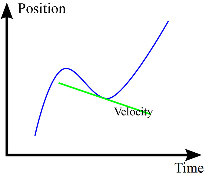
Instantaneous Velocity: The green line shows the tangential line of the position-time curve at a particular time. Its slope is the velocity at that point.
Limit of a Function
The limit of a function is a fundamental concept in calculus and analysis concerning the behavior of a function near a particular input.Learning Objectives
Recognize when a limit does not existKey Takeaways
Key Points
- The function has a limit [latex]L[/latex] at an input [latex]p[/latex] if [latex]f(x)[/latex] is "close" to [latex]L[/latex] whenever [latex]x[/latex] is "close" to [latex]p[/latex].
- To say that [latex]\displaystyle \lim_{x \to p}f(x) = L[/latex] means that [latex]f(x)[/latex] can be made as close as desired to [latex]L[/latex] by making [latex]x[/latex] close enough, but not equal, to [latex]p[/latex].
- For [latex]x[/latex] approaching [latex]p[/latex] from above (right) and below (left), if both of these limits are equal to [latex]L[/latex] then this can be referred to as the limit of [latex]f(x)[/latex] at [latex]p[/latex].
Key Terms
- secant line: a line that (locally) intersects two points on the curve
- function: a relation in which each element of the domain is associated with exactly one element of the co-domain
- derivative: a measure of how a function changes as its input changes
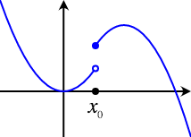
Nonexistence of Limit: The limit as the function approaches [latex]x_0[/latex] from the left does not equal the limit as the function approaches [latex]x_0[/latex] from the right, so the limit of the function at [latex]x_0[/latex] does not exist.
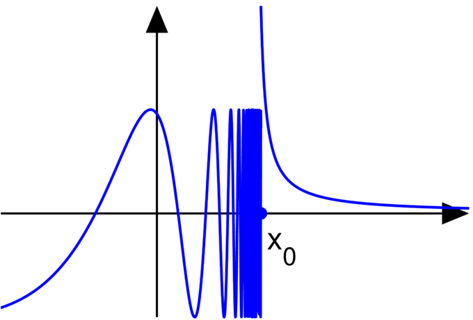
Essential Discontinuity: A graph of the above function, demonstrating that the limit at [latex]x_0[/latex] does not exist.
Calculating Limits Using the Limit Laws
Limits of functions can often be determined using simple laws, such as L'Hôpital's rule and squeeze theorem.Learning Objectives
Calculate a limit using simple laws, such as L'Hôpital's Rule or the squeeze theoremKey Takeaways
Key Points
- L'Hôpital's rule uses derivatives to help evaluate limits involving indeterminate forms.
- When using the L'Hôpital's rule, the differentiation of the numerator and denominator often simplifies the quotient and/or converts it to a determinate form, allowing the limit to be evaluated more easily.
- The squeeze theorem is often used to confirm the limit of a function via comparison with two other functions whose limits are known or easily computed.
Key Terms
- differentiable: having a derivative, said of a function whose domain and co-domain are manifolds
- derivative: a measure of how a function changes as its input changes
L'Hôpital's Rule
L'Hôpital's rule (pronounced "lope-ee-tahl," sometimes spelled l'Hospital's rule with silent "s" and identical pronunciation), also called Bernoulli's rule, uses derivatives to help evaluate limits involving indeterminate forms. Application (or repeated application) of the rule often converts an indeterminate form to a determinate form, allowing easy evaluation of the limit. In its simplest form, l'Hôpital's rule states that if functions [latex]f[/latex] and [latex]g[/latex] are differentiable on an open interval [latex]I[/latex] containing [latex]c[/latex], THEN:- [latex]\displaystyle{\lim_{x \to c}f(x)=\lim_{x \to c}g(x)=0 \text{ or } \pm\infty}[/latex]
- [latex]\displaystyle{\lim_{x\to c}\frac{f'(x)}{g'(x)}}[/latex] exists,
- and, if and only if [latex]g'(x)\neq 0 \text{ for all } x \text{ in } I \text{ } (x \neq c)[/latex], THEN [latex]\displaystyle{\lim_{x\to c}\frac{f(x)}{g(x)} = \lim_{x\to c}\frac{f'(x)}{g'(x)}}[/latex].
The Squeeze Theorem
The squeeze theorem is a technical result that is very important in proofs in calculus and mathematical analysis. It is typically used to confirm the limit of a function via comparison with two other functions whose limits are known or easily computed. The squeeze theorem is formally stated as follows: Let [latex]I[/latex] be an interval having the point [latex]a[/latex] as a limit point. Let [latex]f[/latex], [latex]g[/latex], and [latex]h[/latex] be functions defined on [latex]I[/latex], except possibly at [latex]a[/latex] itself. Suppose that for every [latex]x[/latex] in [latex]I[/latex] not equal to [latex]a[/latex], we have [latex]g(x) \leq f(x) \leq h(x)[/latex], and also suppose that [latex]\lim_{x \to a} g(x) = \lim_{x \to a} h(x) = L[/latex], then [latex]\lim_{x \to a} f(x) = L[/latex].
Squeeze Theorem: [latex]x^2 sin \left ( \frac{1}{x} \right)[/latex]being squeezed by [latex]x^2[/latex] and [latex]-x^2[/latex] in the limit as [latex]x[/latex] approaches [latex]0[/latex].
Precise Definition of a Limit
The [latex](\varepsilon,\delta)[/latex]-definition of limit (the "epsilon-delta definition") is a formalization of the notion of limit.Learning Objectives
Explain the meaning of [latex]\delta[/latex] in the [latex](\varepsilon,\delta)[/latex]-definition of a limit.Key Takeaways
Key Points
- Suppose [latex]f:R \rightarrow R[/latex] is defined on the real line and [latex]p,L \in R[/latex]. It is said the limit of [latex]f[/latex] as [latex]x[/latex] approaches [latex]p[/latex] is [latex]L[/latex] and written [latex]lim_{x} \rightarrow pf(x)=L\lim_{x \to p}f(x) = L [/latex], if the following property holds. (Continued).
- For every real [latex]\varepsilon > 0[/latex], there exists a real [latex]\delta > 0[/latex] such that for all real [latex]x[/latex], [latex]\varepsilon > 0[/latex] [latex]0 < \left | x-p \right | < \delta[/latex] implies [latex]\left | f(x) - L \right | < \varepsilon[/latex]. Note that the value of the limit does not depend on the value of [latex]f(p)[/latex], nor even that [latex]p[/latex] be in the domain of [latex]f[/latex].
- This definition also works for functions with more than one input value.
Key Terms
- infinity: a number that has an infinite numerical value that cannot be counted
- error: the difference between a measured or calculated value and a true one
The [latex](\varepsilon,\delta)[/latex]-Definition
The [latex](\varepsilon,\delta)[/latex]-definition of limit is a formalization of the notion of limit. Suppose [latex]f:R \rightarrow R[/latex] is defined on the real line and [latex]p,L \in R[/latex]. It is said the limit of [latex]f[/latex] as [latex]x[/latex] approaches [latex]p[/latex] is [latex]L[/latex] and written [latex]lim_{x} \rightarrow pf(x)=L\lim_{x \to p}f(x) = L [/latex], if the following property holds:- For every real [latex]\varepsilon > 0[/latex], there exists a real [latex]\delta > 0[/latex] such that for all real [latex]x[/latex], [latex]\varepsilon > 0[/latex] [latex]0 < \left | x-p \right | < \delta[/latex] implies [latex]\left | f(x) - L \right | < \varepsilon[/latex]. Note that the value of the limit does not depend on the value of [latex]f(p)[/latex], nor even that [latex]p[/latex] be in the domain of [latex]f[/latex].

Definitely of a Limit: Whenever a point [latex]x[/latex] is within [latex]\delta[/latex] units of [latex]c[/latex], [latex]f(x)[/latex] is within [latex]\epsilon[/latex] units of [latex]L[/latex].
Example
For an arbitrarily small [latex]\varepsilon[/latex], there always exists a large enough number [latex]N[/latex] such that when [latex]x[/latex] approaches [latex]N[/latex], [latex]\left | f(x)-L \right | < \varepsilon[/latex]. Therefore, the limit of this function at infinity exists.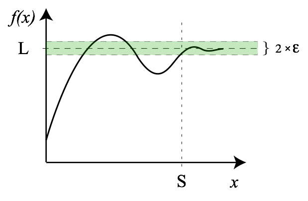
Limit of a Function at Infinity: For an arbitrarily small [latex]\epsilon[/latex], there always exists a large enough number [latex]N[/latex] such that when [latex]x[/latex] approaches [latex]N[/latex], [latex]\left | f(x)-L \right | < \varepsilon[/latex]. Therefore, the limit of this function at infinity exists.
Continuity
A continuous function is a function for which, intuitively, "small" changes in the input result in "small" changes in the output.Learning Objectives
Distinguish between continuous and discontinuous functionsKey Takeaways
Key Points
- If a function is not continuous, it is said to be a "discontinuous function."
- The function [latex]f[/latex] is continuous at some point [latex]c[/latex] of its domain if the limit of [latex]f(x)[/latex] as [latex]x[/latex] approaches [latex]c[/latex] through the domain of [latex]f[/latex] exists and is equal to [latex]f(c)[/latex].
- The function [latex]f[/latex] is said to be continuous if it is continuous at every point of its domain.
Key Terms
- bicontinuous: homomorphic or of structure-preserving mapping
- topology: a branch of mathematics studying those properties of a geometric figure or solid that are not changed by stretching, bending and similar homeomorphisms
- [latex]f[/latex] has to be defined at [latex]c[/latex],
- the limit on the left-hand side of that equation has to exist, and
- the value of this limit must equal [latex]f(c)[/latex].
Finding Limits Algebraically
For a real-valued function expressed in terms of other functions, limit values may be computed via algebraic operations.Learning Objectives
Compute limit values algebraically using properties of limitsKey Takeaways
Key Points
- Algebraic limit theorem states that [latex]\begin{matrix} \lim\limits_{x \to p} & (f(x) + g(x)) & = & \lim\limits_{x \to p} f(x) + \lim\limits_{x \to p} g(x) \\ \lim\limits_{x \to p} & (f(x) - g(x)) & = & \lim\limits_{x \to p} f(x) - \lim\limits_{x \to p} g(x) \\ \lim\limits_{x \to p} & (f(x)\cdot g(x)) & = & \lim\limits_{x \to p} f(x) \cdot \lim\limits_{x \to p} g(x) \\ \lim\limits_{x \to p} & (f(x)/g(x)) & = & {\lim\limits_{x \to p} f(x) / \lim\limits_{x \to p} g(x)} \end{matrix}[/latex].
- In each case above, when the limits on the right do not exist, nonetheless the limit on the left, called an indeterminate form, may still exist.
- When algebraic limit theorem doesn't yield a limit value, corresponding limits might often be determined with L'Hôpital's rule or the Squeeze theorem.
Key Terms
- limit: a value to which a sequence or function converges
- algebraic: containing only numbers, letters, and arithmetic operators
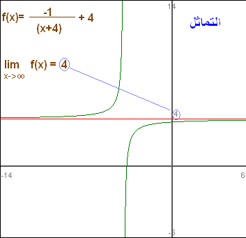
Finding a Limit: The limit of [latex]f(x)= \frac{-1}{(x+4)} + 4[/latex] as [latex]x[/latex] goes to infinity can be segmented down into two parts: the limit of [latex]\frac{−1}{(x+4)}[/latex] and the limit of [latex]4[/latex]. The former is [latex]0[/latex], while the latter is [latex]4[/latex]. Therefore, the limit of [latex]f(x)[/latex] as [latex]x[/latex] goes to infinity is [latex]4[/latex].
Trigonometric Limits
There are several limits of special interest involving trigonometric functions.Learning Objectives
Identify the limits of special interest involving trigonometric functionsKey Takeaways
Key Points
- The limit [latex]\lim_{x \to 0} \frac{\sin x}{x} = 1[/latex] is the most important relation involving limits of trigonometric functions.
- Using the first relation, we can also get [latex]\lim_{x \to 0} \frac{1 - \cos x}{x} = 0[/latex].
- By substituting [latex]t=\frac{1}{x}[/latex] in the first relation, we get [latex]\lim_{x \rightarrow \infty} x \sin \left (\frac{c}{x} \right ) = c[/latex].
Key Terms
- squeeze theorem: theorem obtaining the limit of a function via comparison with two other functions whose limits are known or easily computed
- trigonometric function: any function of an angle expressed as the ratio of two of the sides of a right triangle that has that angle, or various other functions that subtract 1 from this value or subtract this value from 1 (such as the versed sine)
1. [latex]\displaystyle{\lim_{x \to 0} \frac{\sin x}{x} = 1}[/latex]
This limit can be proven with the squeeze theorem. For [latex]0 < x < \frac{ \pi}{2}[/latex], [latex]\sin x < x < \tan x.[/latex] Dividing everything by [latex]\sin x[/latex] yields: [latex-display]1 < \frac{x}{\sin x} < \frac{\tan x}{\sin x}[/latex-display] which reduces to: [latex]\displaystyle{1 < \frac{x}{\sin x} < \frac{1}{\cos x}}[/latex]. Taking the limit of the right-hand side: [latex-display]\displaystyle{\lim_{x \to 0} \left ( \frac{1}{\cos x} \right ) = \frac{1}{1} = 1}[/latex-display] The squeeze theorem tells us that: [latex-display]\displaystyle{\lim_{x \to 0} \left ( \frac{x}{\sin x} \right ) = 1}[/latex-display] Equivalently: [latex-display]\displaystyle{\lim_{x \to 0} \left ( \frac{\sin x}{x} \right ) = 1}[/latex-display]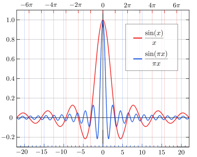
Sinc Function: The normalized sinc (blue, higher frequency) and unnormalized sinc function (red, lower frequency) shown on the same scale.
2. [latex]\displaystyle{\lim_{x \to 0} \frac{1 - \cos x}{x} = 0}[/latex]
This equation can be proven with the first limit and the trigonometric identity [latex]1 - \cos^2 x = \sin^2 x[/latex]. We start with: [latex-display]\displaystyle{\frac{1 - \cos x}{x}}[/latex-display] Multiplying the numerator and denominator by [latex]1 + \cos x[/latex], [latex-display]\displaystyle{\frac{(1−\cos x)(1+\cos x)}{x(1+\cos x)}=\frac{(1−\cos^2x)}{x(1+\cos x)}=\frac{\sin^2x}{x(1+\cos x)}= \frac{\sin x}{x} \cdot \frac{\sin x}{1+\cos x}}[/latex-display] Using the algebraic limit theorem, [latex-display]\displaystyle{\lim_{x \to 0}\left ( \frac{\sin x}{x} \frac{\sin x}{1 + \cos x} \right ) = \left (\lim_{x \to 0} \frac{\sin x}{x} \right ) \left ( \lim_{x \to 0} \frac{\sin x}{1 + \cos x} \right ) = \left (1 \right )\left (\frac{0}{2} \right )= 0}[/latex-display] Therefore: [latex-display]\displaystyle{\lim_{x \to 0} \frac{1 - \cos x}{x} = 0}[/latex-display]3. [latex]\lim_{x \to \infty} x \sin \left(\frac{c}{x}\right) = c[/latex]
This relation can be proven by substituting [latex]t=\frac{1}{x}[/latex] into the first relation we derived: [latex]\displaystyle{\lim_{t \to 0} \left ( \frac{\sin t}{t} \right ) = 1}[/latex].Intermediate Value Theorem
For a real-valued continuous function [latex]f[/latex] on the interval [latex][a,b][/latex] and a number [latex]u[/latex] between [latex]f(a)[/latex] and [latex]f(b)[/latex], there is a [latex]c \in [a,b][/latex] such that [latex]f(c)=u[/latex].Learning Objectives
Use the intermediate value theorem to determine whether a point exists on a continuous functionKey Takeaways
Key Points
- The intermediate value theorem states that for each value between the least upper bound and greatest lower bound of the image of a continuous function there is at least one point in its domain that the function maps to that value.
- The theorem is frequently stated in the following equivalent form: Suppose that [latex]f: [a, b] \to R[/latex] is continuous and that [latex]u[/latex] is a real number satisfying [latex]f(a) < u < f(b)[/latex] or [latex]f(a) > u > f(b)[/latex]. Then for some [latex]c \in [a, b][/latex], [latex]f(c) = u[/latex].
- The theorem depends on (and is actually equivalent to) the completeness of the real numbers.
Key Terms
- real number: a value that represents a quantity along a continuous line
- completeness of the real numbers: completeness implies that there are not any "gaps" or "missing points" in the real number line
- continuous function: a function whose value changes only slightly when its input changes slightly
- Version I: If [latex]f[/latex] is a real-valued continuous function on the interval [latex][a, b][/latex], and [latex]u[/latex] is a number between [latex]f(a)[/latex] and [latex]f(b)[/latex], then there is a [latex]c \in [a, b][/latex] such that [latex]f(c) = u[/latex].
- Version 2: Suppose that [latex]f: [a, b] \to R[/latex] is continuous and that u is a real number satisfying [latex]f(a) < u < f(b)[/latex] or [latex]f(a) > u > f(b)[/latex]. Then for some [latex]c \in [a, b][/latex], [latex]f(c) = u[/latex].
- Version 3: Suppose that [latex]I[/latex] is an interval [latex][a, b][/latex] in the real numbers [latex]\mathbb{R}[/latex] and that [latex]f: I \to R[/latex] is a continuous function. Then the image set [latex]f(I)[/latex] is also an interval, and either it contains [latex][f(a), f(b)][/latex], or it contains [latex][f(b), f(a)][/latex]; that is, [latex]f(I) \supseteq [f(a), f(b)][/latex], or [latex]f(I) \supseteq [f(b), f(a)][/latex].
Infinite Limits
Limits involving infinity can be formally defined using a slight variation of the [latex](\varepsilon, \delta)[/latex]-definition.Learning Objectives
Evaluate the limits of functions as [latex]x[/latex] approaches infinityKey Takeaways
Key Points
- For [latex]f(x)[/latex] a real function, the limit of [latex]f[/latex] as [latex]x[/latex] approaches infinity is [latex]L[/latex], means that for all ε>0\varepsilon > 0, there exists [latex]c[/latex] such that whenever [latex]x > c[/latex], |f(x)−L|<ε|f(x) - L| < \varepsilon.
- For a rational function [latex]f(x)[/latex] of the form [latex]\frac{p(x)}{q(x)}[/latex], there are three basic rules for evaluating limits at infinity, where [latex]p(x)[/latex] and [latex]q(x)[/latex] are polynomials.
- If the limit at infinity exists, it represents a horizontal asymptote at [latex]y = L[/latex].
Key Terms
- definition: a formalization of the notion of the limit of functions
- asymptote: a straight line which a curve approaches arbitrarily closely, as they go to infinity
Infinite Limit: For any arbitrarily small [latex]\varepsilon[/latex], there exists a large enough [latex]N[/latex] such that when [latex]x > N[/latex], [latex]\left | f(x)-2 \right | < \varepsilon[/latex]. Therefore, the limit of this function at infinity exists.
- If the degree of [latex]p[/latex] is greater than the degree of [latex]q[/latex], then the limit is positive or negative infinity depending on the signs of the leading coefficients;
- If the degree of [latex]p[/latex] and [latex]q[/latex] are equal, the limit is the leading coefficient of [latex]p[/latex] divided by the leading coefficient of [latex]q[/latex];
- If the degree of [latex]p[/latex] is less than the degree of [latex]q[/latex], the limit is [latex]0[/latex].
Licenses & Attributions
CC licensed content, Shared previously
- Curation and Revision. Provided by: Boundless.com License: CC BY-SA: Attribution-ShareAlike.
CC licensed content, Specific attribution
- Velocity. Provided by: Wikipedia License: CC BY-SA: Attribution-ShareAlike.
- tangent. Provided by: Wiktionary License: CC BY-SA: Attribution-ShareAlike.
- integral. Provided by: Wiktionary License: CC BY-SA: Attribution-ShareAlike.
- velocity. Provided by: Wiktionary License: CC BY-SA: Attribution-ShareAlike.
- Motion graphs and derivatives. Provided by: Wikipedia License: CC BY: Attribution.
- Limit of a function. Provided by: Wikipedia Located at: https://en.wikipedia.org/wiki/Limit_of_a_function. License: CC BY-SA: Attribution-ShareAlike.
- secant line. Provided by: Wikipedia License: CC BY-SA: Attribution-ShareAlike.
- function. Provided by: Wiktionary License: CC BY-SA: Attribution-ShareAlike.
- derivative. Provided by: Wikipedia License: CC BY-SA: Attribution-ShareAlike.
- Motion graphs and derivatives. Provided by: Wikipedia License: CC BY: Attribution.
- Discontinuity_essential.eps.png. Provided by: Wikipedia License: CC BY-SA: Attribution-ShareAlike.
- Upper_semi.svg. Provided by: Wikipedia License: CC BY-SA: Attribution-ShareAlike.
- Squeeze theorem. Provided by: Wikipedia License: CC BY-SA: Attribution-ShareAlike.
- L'Hu00f4pital's rule. Provided by: Wikipedia License: CC BY-SA: Attribution-ShareAlike.
- differentiable. Provided by: Wiktionary License: CC BY-SA: Attribution-ShareAlike.
- derivative. Provided by: Wikipedia License: CC BY-SA: Attribution-ShareAlike.
- Motion graphs and derivatives. Provided by: Wikipedia License: CC BY: Attribution.
- Discontinuity_essential.eps.png. Provided by: Wikipedia License: CC BY-SA: Attribution-ShareAlike.
- Upper_semi.svg. Provided by: Wikipedia License: CC BY-SA: Attribution-ShareAlike.
- Squeeze theorem. Provided by: Wikipedia License: CC BY: Attribution.
- Limit of a function. Provided by: Wikipedia License: CC BY-SA: Attribution-ShareAlike.
- (u03b5, u03b4)-definition of limit. Provided by: Wikipedia License: CC BY-SA: Attribution-ShareAlike.
- error. Provided by: Wiktionary License: CC BY-SA: Attribution-ShareAlike.
- infinity. Provided by: Wiktionary License: CC BY-SA: Attribution-ShareAlike.
- Motion graphs and derivatives. Provided by: Wikipedia License: CC BY: Attribution.
- Discontinuity_essential.eps.png. Provided by: Wikipedia License: CC BY-SA: Attribution-ShareAlike.
- Upper_semi.svg. Provided by: Wikipedia License: CC BY-SA: Attribution-ShareAlike.
- Squeeze theorem. Provided by: Wikipedia License: CC BY: Attribution.
- (u03b5, u03b4)-definition of limit. Provided by: Wikipedia License: CC BY: Attribution.
- Limit of a function. Provided by: Wikipedia License: CC BY: Attribution.
- Continuous function. Provided by: Wikipedia License: CC BY-SA: Attribution-ShareAlike.
- bicontinuous. Provided by: Wiktionary License: CC BY-SA: Attribution-ShareAlike.
- topology. Provided by: Wiktionary License: CC BY-SA: Attribution-ShareAlike.
- Motion graphs and derivatives. Provided by: Wikipedia License: CC BY: Attribution.
- Discontinuity_essential.eps.png. Provided by: Wikipedia License: CC BY-SA: Attribution-ShareAlike.
- Upper_semi.svg. Provided by: Wikipedia License: CC BY-SA: Attribution-ShareAlike.
- Squeeze theorem. Provided by: Wikipedia License: CC BY: Attribution.
- (u03b5, u03b4)-definition of limit. Provided by: Wikipedia License: CC BY: Attribution.
- Limit of a function. Provided by: Wikipedia License: CC BY: Attribution.
- Limit of a function. Provided by: Wikipedia License: CC BY-SA: Attribution-ShareAlike.
- algebraic. Provided by: Wiktionary License: CC BY-SA: Attribution-ShareAlike.
- limit. Provided by: Wiktionary License: CC BY-SA: Attribution-ShareAlike.
- Motion graphs and derivatives. Provided by: Wikipedia License: CC BY: Attribution.
- Discontinuity_essential.eps.png. Provided by: Wikipedia Located at: https://en.wikipedia.org/wiki/Limit_of_a_function. License: CC BY-SA: Attribution-ShareAlike.
- Upper_semi.svg. Provided by: Wikipedia License: CC BY-SA: Attribution-ShareAlike.
- Squeeze theorem. Provided by: Wikipedia License: CC BY: Attribution.
- (u03b5, u03b4)-definition of limit. Provided by: Wikipedia License: CC BY: Attribution.
- Limit of a function. Provided by: Wikipedia License: CC BY: Attribution.
- Limit of a function. Provided by: Wikipedia License: CC BY: Attribution.
- Limit of a function. Provided by: Wikipedia License: CC BY-SA: Attribution-ShareAlike.
- squeeze theorem. Provided by: Wikipedia License: CC BY-SA: Attribution-ShareAlike.
- trigonometric function. Provided by: Wiktionary License: CC BY-SA: Attribution-ShareAlike.
- Motion graphs and derivatives. Provided by: Wikipedia License: CC BY: Attribution.
- Discontinuity_essential.eps.png. Provided by: Wikipedia License: CC BY-SA: Attribution-ShareAlike.
- Upper_semi.svg. Provided by: Wikipedia License: CC BY-SA: Attribution-ShareAlike.
- Squeeze theorem. Provided by: Wikipedia License: CC BY: Attribution.
- (u03b5, u03b4)-definition of limit. Provided by: Wikipedia License: CC BY: Attribution.
- Limit of a function. Provided by: Wikipedia License: CC BY: Attribution.
- Limit of a function. Provided by: Wikipedia License: CC BY: Attribution.
- Si_sinc.svg. Provided by: Wikipedia License: CC BY-SA: Attribution-ShareAlike.
- continuous function. Provided by: Wiktionary License: CC BY-SA: Attribution-ShareAlike.
- real number. Provided by: Wiktionary License: CC BY-SA: Attribution-ShareAlike.
- Intermediate value theorem. Provided by: Wikipedia License: CC BY-SA: Attribution-ShareAlike.
- completeness of the real numbers. Provided by: Wikipedia License: CC BY-SA: Attribution-ShareAlike.
- Motion graphs and derivatives. Provided by: Wikipedia License: CC BY: Attribution.
- Discontinuity_essential.eps.png. Provided by: Wikipedia License: CC BY-SA: Attribution-ShareAlike.
- Upper_semi.svg. Provided by: Wikipedia License: CC BY-SA: Attribution-ShareAlike.
- Squeeze theorem. Provided by: Wikipedia License: CC BY: Attribution.
- (u03b5, u03b4)-definition of limit. Provided by: Wikipedia License: CC BY: Attribution.
- Limit of a function. Provided by: Wikipedia License: CC BY: Attribution.
- Limit of a function. Provided by: Wikipedia License: CC BY: Attribution.
- Si_sinc.svg. Provided by: Wikipedia License: CC BY-SA: Attribution-ShareAlike.
- Limit of a function. Provided by: Wikipedia License: CC BY-SA: Attribution-ShareAlike.
- asymptote. Provided by: Wiktionary License: CC BY-SA: Attribution-ShareAlike.
- definition. Provided by: Wiktionary License: CC BY-SA: Attribution-ShareAlike.
- Motion graphs and derivatives. Provided by: Wikipedia License: CC BY: Attribution.
- Discontinuity_essential.eps.png. Provided by: Wikipedia License: CC BY-SA: Attribution-ShareAlike.
- Upper_semi.svg. Provided by: Wikipedia License: CC BY-SA: Attribution-ShareAlike.
- Squeeze theorem. Provided by: Wikipedia License: CC BY: Attribution.
- (u03b5, u03b4)-definition of limit. Provided by: Wikipedia License: CC BY: Attribution.
- Limit of a function. Provided by: Wikipedia License: CC BY: Attribution.
- Limit of a function. Provided by: Wikipedia License: CC BY: Attribution.
- Si_sinc.svg. Provided by: Wikipedia Located at: https://en.wikipedia.org/wiki/Sinc_function. License: CC BY-SA: Attribution-ShareAlike.
- Limit of a function. Provided by: Wikipedia License: CC BY: Attribution.
