Integrals
Antiderivatives
An antiderivative is a differentiable function [latex]F[/latex] whose derivative is equal to [latex]f[/latex] (i.e., [latex]F' = f[/latex]).Learning Objectives
Calculate the antiderivative (aka the indefinite integral) for a given functionKey Takeaways
Key Points
- The process of solving for antiderivatives is called antidifferentiation, and its opposite operation is called differentiation, which is the process of finding a derivative.
- Antiderivatives are related to definite integrals through the fundamental theorem of calculus: the definite integral of a function over an interval is equal to the difference between the values of an antiderivative evaluated at the endpoints of the interval.
- The graphs of antiderivatives of a given function are vertical translations of each other, with each graph's location depending upon the value of constant [latex]C[/latex].
Key Terms
- derivative: a measure of how a function changes as its input changes
- definite integral: the integral of a function between an upper and lower limit
Area and Distances
Defined integrals are used in many practical situations that require distance, area, and volume calculations.Learning Objectives
Apply integration to calculate problems about the area under a graph, or the distance of an arcKey Takeaways
Key Points
- The definite integral [latex]\int_{a}^{b}f(x)dx[/latex] is defined informally to be the area of the region in the [latex]xy[/latex]-plane bound by the graph of [latex]f[/latex], the [latex]x[/latex]-axis, and the vertical lines [latex]x = a [/latex] and [latex]x=b[/latex], such that the area above the [latex]x[/latex]-axis adds to the total, and the area below the [latex]x[/latex]-axis subtracts from the total.
- According to the fundamental theorem of calculus: if [latex]f[/latex] is a continuous real-valued function defined on a closed interval [latex][a,b][/latex], then, once an antiderivative [latex]F[/latex] of [latex]f[/latex] is known, the definite integral of [latex]f[/latex] over that interval is given by [latex]\int_{a}^{b}f(x)dx = F(b) - F(a)[/latex].
- When practical approximation does not provide precise enough results for distance, area, and volume calculations, integration must be performed.
Key Terms
- antiderivative: an indefinite integral
- integration: the operation of finding the region in the [latex]xy[/latex]-plane bound by a given function
- definite integral: the integral of a function between an upper and lower limit
Area
To start off, consider the curve [latex]y = f(x)[/latex] between [latex]0[/latex] and [latex]x=1[/latex] with [latex]f(x) = \sqrt{x}.[/latex] We ask, "What is the area under the function [latex]f[/latex], over the interval from [latex]0[/latex] to [latex]1[/latex]? " and call this (yet unknown) area the integral of [latex]f[/latex]. The notation for this integral will be: [latex-display]\displaystyle{\int_{0}^{1} \sqrt{x} dx}[/latex-display] As a first approximation, look at the unit square given by the sides [latex]x = 0[/latex] to [latex]x = 1[/latex], [latex]y = f(0) = 0[/latex], and [latex]y = f(1) = 1[/latex]. Its area is exactly [latex]1[/latex]. As it is, the true value of the integral must be somewhat less. Decreasing the width of the approximation rectangles should yield a better result, so we will cross the interval in five steps, using the approximation points [latex]0[/latex], [latex]\frac{1}{5}[/latex], [latex]\frac{2}{5}[/latex], and so on, up to [latex]1[/latex]. Fit a box for each step using the right end height of each curve piece, thus obtaining [latex]\sqrt{\frac{1}{5}}[/latex], [latex]\sqrt{\frac{2}{5}}[/latex], and so on, up to[latex]\sqrt{1} = 1[/latex]. Summing the areas of these rectangles, we get a better approximation for the sought integral, namely: [latex-display]\displaystyle{\sqrt{\frac{1}{5}} \left ( \frac{1}{5} - 0 \right ) + \sqrt{\frac{2}{5}} \left ( \frac{2}{5} - \frac{1}{5} \right ) + \cdots + \sqrt{\frac{5}{5}} \left ( \frac{5}{5} - \frac{4}{5} \right ) \approx 0.7497}[/latex-display] Notice that we are taking a finite sum of many function values of [latex]f[/latex], multiplied with the differences of two subsequent approximation points. We can easily see that the approximation is still too large. Using more steps produces a closer approximation, but will never be exact: replacing the [latex]5[/latex] subintervals by twelve as depicted, we will get an approximate value for the area of [latex]0.6203[/latex], which is too small. The key idea is the transition from adding a finite number of differences of approximation points multiplied by their respective function values to using an infinite number of fine, or infinitesimal, steps.
Integral Approximation: Approximations to integral of [latex]\sqrt x[/latex] from [latex]0[/latex] to [latex]1[/latex], with yellow [latex]5[/latex] right samples (above) and green [latex]12[/latex] left samples (below).
Distance (Finding arc length by Integrating)
If you know the velocity [latex]v(t) [/latex] of an object as a function of time, you can simply integrate [latex]v(t) [/latex] over time to calculate the distance the object traveled. Since this is equivalent to evaluating the area under the curve [latex]v(t) [/latex], we will not discuss more on this. However, you can also use integrals to calculate length—for example, the length of an arc described by a function [latex]y = f(x)[/latex]. Consider an infinitesimal part of the curve [latex]ds[/latex] on the curve (or consider this as a limit in which the change in [latex]s[/latex] approaches [latex]ds[/latex]). According to Pythagoras's theorem, [latex]ds^2=dx^2+dy^2[/latex], from which we can determine: [latex-display]\displaystyle{\frac{ds^2}{dx^2}=1+\frac{dy^2}{dx^2}}[/latex-display] [latex-display]\displaystyle{ds=\sqrt{1+\left(\frac{dy}{dx}\right)^2}dx}[/latex-display] [latex-display]\displaystyle{s = \int_{a}^{b} \sqrt { 1 + [f'(x)]^2 }\, dx}[/latex-display]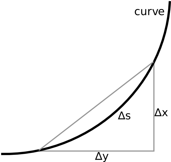
Calculating arc length: For a small piece of curve, [latex]\Delta s[/latex] can be approximated with the Pythagorean theorem.
Example
For the following curve described by the parameter [latex]t[/latex]: [latex-display]\begin{cases} y = t^5 \\ x = t^3 \end{cases}[/latex-display] the arc length integral for values of [latex]t[/latex] from [latex]-1[/latex] to [latex]1[/latex] is: [latex-display]\displaystyle{\int_{-1}^1 \sqrt{(3t^2)^2 + (5t^4)^2}\,dt}[/latex-display] [latex-display]\displaystyle{= \int_{-1}^1 \sqrt{9t^4 + 25t^8}\,dt}[/latex-display]
Definite Integral: A definite integral of a function can be represented as the signed area of the region bound by its graph.
The Definite Integral
A definite integral is the area of the region in the [latex]xy[/latex]-plane bound by the graph of [latex]f[/latex], the [latex]x[/latex]-axis, and the vertical lines [latex]x=a[/latex] and [latex]x=b[/latex].Learning Objectives
Compute the definite integral of a function over a set intervalKey Takeaways
Key Points
- Integration is an important concept in mathematics and—together with its inverse, differentiation —is one of the two main operations in calculus.
- Integration is connected with differentiation through the fundamental theorem of calculus: if [latex]f[/latex] is a continuous real-valued function defined on a closed interval [latex][a, b][/latex], then, once an antiderivative [latex]F[/latex] of [latex]f[/latex] is known, the definite integral of [latex]f[/latex] over that interval is given by [latex]\int_{a}^{b}f(x)dx = F(b) - F(a)[/latex].
- Definite integrals appear in many practical situations, and their actual calculation is important in the type of precision engineering (of any discipline) that requires exact and rigorous values.
Key Terms
- definite integral: the integral of a function between an upper and lower limit
- integration: the operation of finding the region in the [latex]xy[/latex]-plane bound by the function
- antiderivative: an indefinite integral
Definite Integral: A definite integral of a function can be represented as the signed area of the region bounded by its graph.
The Fundamental Theorem of Calculus
The fundamental theorem of calculus is a theorem that links the concept of the derivative of a function to the concept of the integral.Learning Objectives
Define the first and second fundamental theorems of calculusKey Takeaways
Key Points
- The first part of the theorem shows that an indefinite integration can be reversed by differentiation.
- The second part allows one to compute the definite integral of a function by using any one of its infinitely many antiderivatives.
- The second part of the theorem has invaluable practical applications because it markedly simplifies the computation of definite integrals.
Key Terms
- antiderivative: an indefinite integral
- derivative: a measure of how a function changes as its input changes
- definite integral: the integral of a function between an upper and lower limit

The Fundamental Theorem of Calculus: We can see from this picture that the Fundamental Theorem of Calculus works. By definition, the derivative of [latex]A(x)[/latex] is equal to [latex]\frac{A(x+h)−A(x)}{h}[/latex] as [latex]h[/latex] tends to zero. By replacing the numerator, [latex]A(x+h)−A(x)[/latex], by [latex]hf(x)[/latex] and dividing by [latex]h[/latex], [latex]f(x)[/latex] is obtained. Taking the limit as [latex]h[/latex] tends to zero completes the proof of the Fundamental Theorem of Calculus.
Indefinite Integrals and the Net Change Theorem
An indefinite integral is defined as [latex]\int f(x)dx = F(x)+ C[/latex], where [latex]F[/latex] satisfies [latex]F'(x) = f(x)[/latex] and where [latex]C[/latex] is any constant.Learning Objectives
Apply the basic properties of indefinite integrals, including the constant, sum, and difference rulesKey Takeaways
Key Points
- The constant rule for indefinite integrals: [latex]\int cf(x)dx = c\int f(x)dx[/latex]
- The sum rule for indefinite integrals: [latex]\int (f(x)+ g(x)) dx = \int f(x)dx + \int g(x)dx[/latex]
- The difference rule for indefinite integrals: [latex]\int (f(x)- g(x)) dx = \int f(x)dx - \int g(x)dx[/latex]
- The integral of a rate of change is the net change (displacement for position functions ): [latex]\int_{a}^{b} f(x)dx = f(b) - f(a)[/latex]
Key Terms
- antiderivative: an indefinite integral
- definite integral: the integral of a function between an upper and lower limit
- integral: also sometimes called antiderivative; the limit of the sums computed in a process in which the domain of a function is divided into small subsets and a possibly nominal value of the function on each subset is multiplied by the measure of that subset, all these products then being summed
Indefinite Integrals and Antiderivatives
As you remember from the atoms on antiderivatives, [latex]F[/latex] is said to be an antiderivative of [latex]f[/latex] if [latex]F'(x) = f(x)[/latex]. However, [latex]F[/latex] is not the only antiderivative. We can add any constant [latex]C[/latex] to [latex]F[/latex] without changing the derivative. With this in mind, we define the indefinite integral as follows: [latex]\int f(x)dx = F(x)+ C[/latex], where [latex]F[/latex] satisfies [latex]F'(x) = f(x)[/latex] and [latex]C[/latex] is any constant. [latex]f(x)[/latex], the function being integrated, is known as the integrand. Note that the indefinite integral yields a family of functions. For example, the function [latex]F(x) = \frac{x^3}{3}[/latex] is an antiderivative of [latex]f(x) = x^2[/latex]. Since the derivative of a constant is zero, [latex]x^2[/latex] will have an infinite number of antiderivatives, such as [latex]\left ( \frac{x^3}{3} \right ) + 0[/latex], [latex]\left ( \frac{x^3}{3} \right ) + 7[/latex], [latex]\left ( \frac{x^3}{3} \right ) - 42[/latex],[latex]\left ( \frac{x^3}{3} \right ) + 293[/latex], etc. Therefore, all the antiderivatives of [latex]x^2[/latex] can be obtained by changing the value of [latex]C[/latex] in [latex]F(x) = \left ( \frac{x^3}{3} \right ) + C[/latex], where [latex]C[/latex] is an arbitrary constant known as the constant of integration. Essentially, the graphs of antiderivatives of a given function are vertical translations of each other, with each graph's location depending upon the value of [latex]C[/latex].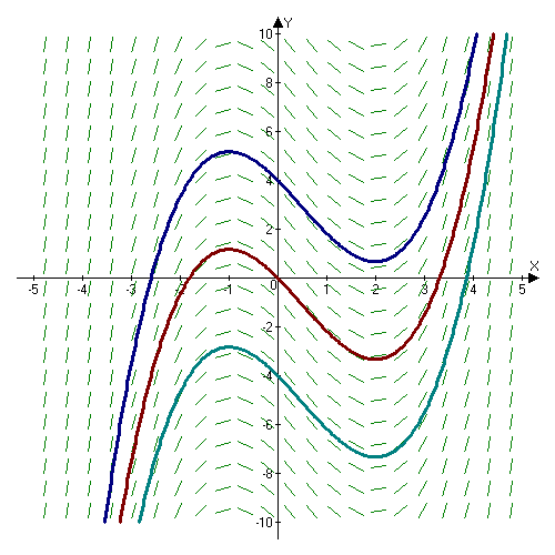
Slope Field: The slope field of [latex]F(x) = \left ( \frac{x^3}{3} \right ) - \left ( \frac{x^2}{2} \right )-x+c[/latex], showing three of the infinitely many solutions that can be produced by varying the arbitrary constant [latex]C[/latex].
The Constant Rule for Indefinite Integrals
[latex-display]\int cf(x)dx = c\int f(x)dx[/latex-display]The Sum Rule for Indefinite Integrals
[latex-display]\int (f(x)+ g(x)) dx = \int f(x)dx + \int g(x)dx[/latex-display]The Difference Rule for Indefinite Integrals
[latex-display]\int (f(x)- g(x)) dx = \int f(x)dx - \int g(x)dx[/latex-display]Definite Integrals and the Net Change Theorem
Integrating over a specified domain yields what is called a " definite integral " (in that the domain is defined). Integrating over a domain [latex]D[/latex] is written as [latex]\int_{a}^{b} f(x)dx[/latex] if the domain is an interval [latex][a, b][/latex] of [latex]x[/latex]. Such a problem can be solved using the net change theorem, which states that the integral of a rate of change is the net change (displacement for position functions): [latex-display]\displaystyle{\int_{a}^{b} f(x)dx = f(b) - f(a)}[/latex-display] Basically, the theorem states that the integral of or [latex]F'[/latex] from [latex]a[/latex] to [latex]b[/latex] is the area between [latex]a[/latex] and [latex]b[/latex], or the difference in area from the position of [latex]f(a)[/latex] to the position of [latex]f(b)[/latex]. This can be applied to find values such as volume, concentration, density, population, cost, and velocity.The Substitution Rule
Integration by substitution is an important tool for mathematicians used to find integrals and antiderivatives.Learning Objectives
Use [latex]u[/latex]-substitution (the substitution rule) to find the antiderivative of more complex functionsKey Takeaways
Key Points
- The substitution [latex]x = g(t)[/latex] yields [latex]\frac{dx}{dt} = g'(t)[/latex] and therefore, formally, [latex]dx = g'(t)dt[/latex], which is the required substitution for [latex]dx[/latex].
- [latex]u[/latex]-substitution (also called [latex]w[/latex]-substitution) is used to simplify a given integral.
- Substitution can be used to determine antiderivatives.
Key Terms
- integration: the operation of finding the region in the [latex]x[/latex]-[latex]y[/latex] plane bound by the function
- antiderivative: an indefinite integral
Definite Integral: A definite integral of a function can be represented as the signed area of the region bounded by its graph.
Further Transcendental Functions
A transcendental function is a function that is not algebraic.Learning Objectives
Identify a transcendental function as one that cannot be expressed as the finite sequence of an algebraic operationKey Takeaways
Key Points
- Transcendental functions cannot be expressed as a solution of a polynomial equation whose coefficients are themselves polynomials with rational coefficients.
- Examples of transcendental functions include the exponential function, the logarithm, and the trigonometric functions.
- Transcendental functions can be an easy-to-spot source of dimensional errors.
Key Terms
- polynomial: an expression consisting of a sum of a finite number of terms, each term being the product of a constant coefficient and one or more variables raised to a non-negative integer power
- trigonometric function: any function of an angle expressed as the ratio of two of the sides of a right triangle that has that angle, or various other functions that subtract 1 from this value or subtract this value from 1 (such as the versed sine)
- exponential function: any function in which an independent variable is in the form of an exponent; they are the inverse functions of logarithms
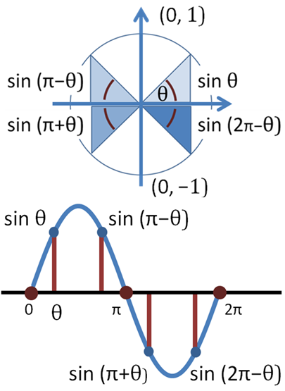
Trigonometric Functions: Top panel: Trigonometric function sinθ for selected angles [latex]\theta[/latex], [latex]\pi - \theta[/latex], [latex]\pi + \theta[/latex], and [latex]2\pi - \theta[/latex] in the four quadrants. Bottom panel: Graph of sine function versus angle.
Numerical Integration
Numerical integration is a method of approximating the value of a definite integral.Learning Objectives
Solve for the definite integral of a continuous function over a closed intervalKey Takeaways
Key Points
- Numerical methods of approximation are useful when the integral is difficult to solve by hand.
- Some methods of numerical integration include the rectangle rule and the trapezoidal rule.
- Since computers cannot solve integrals by hand and are very fast at arithmetic, they use numerical methods to solve integrals.
Key Terms
- approximation: An imprecise solution or result that is adequate for a defined purpose.
- definite integral: the integral of a function between an upper and lower limit
Definite Integral: A definite integral of a function can be represented as the signed area of the region bounded by its graph.

Rectangle Rule: Illustration of the rectangle rule of numerical integration. The value of [latex]f(x)[/latex] is taken to be constant around a point and the integral is calculated by adding up the areas of the rectangles.

Trapezoidal Rule: Illustration of the trapezoidal rule.
Licenses & Attributions
CC licensed content, Shared previously
- Curation and Revision. Provided by: Boundless.com License: CC BY-SA: Attribution-ShareAlike.
CC licensed content, Specific attribution
- Antiderivatives. Provided by: Wikipedia License: CC BY-SA: Attribution-ShareAlike.
- derivative. Provided by: Wikipedia License: CC BY-SA: Attribution-ShareAlike.
- definite integral. Provided by: Wiktionary License: CC BY-SA: Attribution-ShareAlike.
- Definite integral. Provided by: Wikipedia License: CC BY-SA: Attribution-ShareAlike.
- integration. Provided by: Wiktionary License: CC BY-SA: Attribution-ShareAlike.
- antiderivative. Provided by: Wiktionary License: CC BY-SA: Attribution-ShareAlike.
- definite integral. Provided by: Wiktionary License: CC BY-SA: Attribution-ShareAlike.
- Arc length. Provided by: Wikipedia License: CC BY: Attribution.
- Provided by: Wikimedia License: CC BY-SA: Attribution-ShareAlike.
- Provided by: Wikimedia License: CC BY-SA: Attribution-ShareAlike.
- Definite integral. Provided by: Wikipedia License: CC BY-SA: Attribution-ShareAlike.
- antiderivative. Provided by: Wiktionary License: CC BY-SA: Attribution-ShareAlike.
- integration. Provided by: Wiktionary Located at: https://en.wiktionary.org/wiki/integration. License: CC BY-SA: Attribution-ShareAlike.
- definite integral. Provided by: Wiktionary License: CC BY-SA: Attribution-ShareAlike.
- Arc length. Provided by: Wikipedia License: CC BY: Attribution.
- Provided by: Wikimedia License: CC BY-SA: Attribution-ShareAlike.
- Provided by: Wikimedia License: CC BY-SA: Attribution-ShareAlike.
- Provided by: Wikimedia License: CC BY-SA: Attribution-ShareAlike.
- Fundamental theorem of calculus. Provided by: Wikipedia License: CC BY-SA: Attribution-ShareAlike.
- antiderivative. Provided by: Wiktionary License: CC BY-SA: Attribution-ShareAlike.
- derivative. Provided by: Wikipedia License: CC BY-SA: Attribution-ShareAlike.
- definite integral. Provided by: Wiktionary License: CC BY-SA: Attribution-ShareAlike.
- Arc length. Provided by: Wikipedia License: CC BY: Attribution.
- Provided by: Wikimedia License: CC BY-SA: Attribution-ShareAlike.
- Provided by: Wikimedia License: CC BY-SA: Attribution-ShareAlike.
- Provided by: Wikimedia License: CC BY-SA: Attribution-ShareAlike.
- Provided by: Wikimedia License: CC BY-SA: Attribution-ShareAlike.
- Antiderivative. Provided by: Wikipedia License: CC BY-SA: Attribution-ShareAlike.
- Calculus/Indefinite integral. Provided by: Wikibooks License: CC BY-SA: Attribution-ShareAlike.
- Integral. Provided by: Wikipedia License: CC BY-SA: Attribution-ShareAlike.
- integral. Provided by: Wiktionary License: CC BY-SA: Attribution-ShareAlike.
- antiderivative. Provided by: Wiktionary License: CC BY-SA: Attribution-ShareAlike.
- definite integral. Provided by: Wiktionary License: CC BY-SA: Attribution-ShareAlike.
- Arc length. Provided by: Wikipedia License: CC BY: Attribution.
- Provided by: Wikimedia License: CC BY-SA: Attribution-ShareAlike.
- Provided by: Wikimedia License: CC BY-SA: Attribution-ShareAlike.
- Provided by: Wikimedia License: CC BY-SA: Attribution-ShareAlike.
- Provided by: Wikimedia License: CC BY-SA: Attribution-ShareAlike.
- Provided by: Wikimedia License: CC BY-SA: Attribution-ShareAlike.
- Substitution rule. Provided by: Wikipedia License: CC BY-SA: Attribution-ShareAlike.
- Substitution rule. Provided by: Wikipedia License: CC BY-SA: Attribution-ShareAlike.
- integration. Provided by: Wiktionary License: CC BY-SA: Attribution-ShareAlike.
- antiderivative. Provided by: Wiktionary License: CC BY-SA: Attribution-ShareAlike.
- Arc length. Provided by: Wikipedia License: CC BY: Attribution.
- Provided by: Wikimedia License: CC BY-SA: Attribution-ShareAlike.
- Provided by: Wikimedia License: CC BY-SA: Attribution-ShareAlike.
- Provided by: Wikimedia License: CC BY-SA: Attribution-ShareAlike.
- Provided by: Wikimedia License: CC BY-SA: Attribution-ShareAlike.
- Provided by: Wikimedia License: CC BY-SA: Attribution-ShareAlike.
- Provided by: Wikimedia License: CC BY-SA: Attribution-ShareAlike.
- Transcendental functions. Provided by: Wikipedia Located at: https://en.wikipedia.org/wiki/Transcendental_functions. License: CC BY-SA: Attribution-ShareAlike.
- polynomial. Provided by: Wiktionary License: CC BY-SA: Attribution-ShareAlike.
- exponential function. Provided by: Wiktionary License: CC BY-SA: Attribution-ShareAlike.
- trigonometric function. Provided by: Wiktionary License: CC BY-SA: Attribution-ShareAlike.
- Arc length. Provided by: Wikipedia License: CC BY: Attribution.
- Provided by: Wikimedia License: CC BY-SA: Attribution-ShareAlike.
- Provided by: Wikimedia License: CC BY-SA: Attribution-ShareAlike.
- Provided by: Wikimedia License: CC BY-SA: Attribution-ShareAlike.
- Provided by: Wikimedia License: CC BY-SA: Attribution-ShareAlike.
- Provided by: Wikimedia License: CC BY-SA: Attribution-ShareAlike.
- Provided by: Wikimedia License: CC BY-SA: Attribution-ShareAlike.
- Provided by: Wikimedia License: CC BY-SA: Attribution-ShareAlike.
- Definite integral. Provided by: Wikipedia License: CC BY-SA: Attribution-ShareAlike.
- Numerical integration. Provided by: Wikipedia License: CC BY-SA: Attribution-ShareAlike.
- Numerical integration. Provided by: Wikipedia License: CC BY-SA: Attribution-ShareAlike.
- approximation. Provided by: Wiktionary License: CC BY-SA: Attribution-ShareAlike.
- definite integral. Provided by: Wiktionary License: CC BY-SA: Attribution-ShareAlike.
- Arc length. Provided by: Wikipedia License: CC BY: Attribution.
- Provided by: Wikimedia License: CC BY-SA: Attribution-ShareAlike.
- Provided by: Wikimedia License: CC BY-SA: Attribution-ShareAlike.
- Provided by: Wikimedia License: CC BY-SA: Attribution-ShareAlike.
- Provided by: Wikimedia License: CC BY-SA: Attribution-ShareAlike.
- Provided by: Wikimedia License: CC BY-SA: Attribution-ShareAlike.
- Provided by: Wikimedia License: CC BY-SA: Attribution-ShareAlike.
- Provided by: Wikimedia License: CC BY-SA: Attribution-ShareAlike.
- Numerical integration. Provided by: Wikipedia License: CC BY: Attribution.
- Provided by: Wikimedia License: CC BY-SA: Attribution-ShareAlike.
- Numerical integration. Provided by: Wikipedia License: CC BY: Attribution.
