Differential Equations
Solving Differential Equations
Differential equations are solved by finding the function for which the equation holds true.Learning Objectives
Calculate the order and degree of a differential equation.Key Takeaways
Key Points
- The order of a differential equation is determined by the highest-order derivative; the degree is determined by the highest power on a variable.
- The higher the order of the differential equation, the more arbitrary constants need to be added to the general solution. A first-order equation will have one, a second-order two, and so on.
- A particular solution can be found by assigning values to the arbitrary constants to match any given constraints.
Key Terms
- function: a relation in which each element of the domain is associated with exactly one element of the co-domain
- derivative: a measure of how a function changes as its input changes
Solving a Differential Equation: A Simple Example
Take the following differential equation: [latex-display]\displaystyle{f(x) + f'(x) =0}[/latex-display] This equation states that [latex]f(x)[/latex] is equal to the negative of its derivative. You may recall that one function that satisfies this property is [latex]f(x)[/latex] = [latex]e^{-x}[/latex]. The derivative of [latex-display]f(x)[/latex-display] equals -[latex]e^{-x}[/latex] i.e. -[latex]f(x)[/latex] so this function solves the differential equation. A complete solution contains the same number of arbitrary constants as the order of the original equation. (This is because, in order to solve a differential equation of the [latex]n[/latex]th order, you will integrate [latex]n[/latex] times, each time adding a new arbitrary constant.) Since our example above is a first-order equation, it will have just one arbitrary constant in the complete solution. Therefore, the general solution is [latex]f(x) = Ce^{-x}[/latex], where [latex]C[/latex] stands for an arbitrary constant. You can see that the differential equation still holds true with this constant. For a specific solution, replace the constants in the general solution with actual numeric values.Models Using Differential Equations
Differential equations can be used to model a variety of physical systems.Learning Objectives
Give examples of systems that can be modeled with differential equationsKey Takeaways
Key Points
- Many systems can be well understood through differential equations.
- Mathematical models of differential equations can be used to solve problems and generate models.
- An example of such a model is the differential equation governing radioactive decay.
Key Terms
- differential equation: an equation involving the derivatives of a function
- decay: To change by undergoing fission, by emitting radiation, or by capturing or losing one or more electrons.
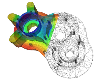
Visual Model of Heat Transfer: Visualization of heat transfer in a pump casing, created by solving the heat equation. Heat is being generated internally in the casing and being cooled at the boundary, providing a steady state temperature distribution.
Direction Fields and Euler's Method
Direction fields and Euler's method are ways of visualizing and approximating the solutions to differential equations.Learning Objectives
Describe application of direction fields and Euler's method to approximate the solutions to differential equationsKey Takeaways
Key Points
- Direction fields, or slope fields, are graphs where each point [latex](x,y)[/latex] has a slope.
- Euler's method is a way of approximating solutions to differential equations by assuming that the slope at a point is the same as the slope between that point and the next point.
- Euler's method gives approximate solutions to differential equations, and the smaller the distance between the chosen points, the more accurate the result.
Key Terms
- tangent: a straight line touching a curve at a single point without crossing it there
- differential equation: an equation involving the derivatives of a function
- normalize: (in mathematics) to divide a vector by its magnitude to produce a unit vector
Direction Fields
Direction fields, also known as slope fields, are graphical representations of the solution to a first order differential equation. They can be achieved without solving the differential equation analytically, and serve as a useful way to visualize the solutions. The slope field is traditionally defined for differential equations of the following form: [latex-display]y'=f(x)[/latex-display] It can be viewed as a creative way to plot a real-valued function of two real variables as a planar picture.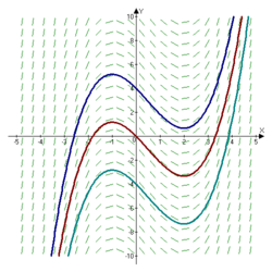
Example slope field: The slope field of [latex]\frac{dy}{dx}=x^2-x-2[/latex], with the blue, red, and turquoise lines being [latex]\frac{x^3}{3}-\frac{x^2}{2}-2x+4[/latex], [latex]\frac{x^3}{3}-\frac{x^2}{2}-2x[/latex], and [latex]\frac{x^3}{3}-\frac{x^2}{2}-2x-4[/latex], respectively.
Euler's Method
Consider the problem of calculating the shape of an unknown curve which starts at a given point and satisfies a given differential equation. Here, a differential equation can be thought of as a formula by which the slope of the tangent line to the curve can be computed at any point on the curve, once the position of that point has been calculated.The idea is that while the curve is initially unknown, its starting point, which we denote by [latex]A_0[/latex], is known (see ). Then, from the differential equation, the slope to the curve at [latex]A_0[/latex] can be computed, and thus, the tangent line.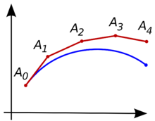
Euler's Method: Illustration of the Euler method. The unknown curve is in blue and its polygonal approximation is in red.
Separable Equations
Separable differential equations are equations wherein the variables can be separated.Learning Objectives
Identify steps necessary to solve separable equationsKey Takeaways
Key Points
- Separable equations are of the form [latex]M(y)\frac{dy}{dx}=N(x)[/latex].
- Separable equations are among the easiest differential equations to solve.
- To solve, collect all terms that contain the same variables to one side and integrate through.
Key Terms
- fraction: a ratio of two numbers, the numerator and the denominator; usually written one above the other and separated by a horizontal bar
- differential equation: an equation involving the derivatives of a function
- derivative: a measure of how a function changes as its input changes
- Multiply and divide to get rid of any fractions.
- Combine any terms involving the same differential into one term.
- Integrate each component on its own, and don't forget to add constants to equations after integrating. This ensures that the solution is of the general form.
- Finally, simplify the expression (i.e., combine all possible terms, rewrite any logarithmic terms in exponent form, and express any arbitrary constants in the most simple terms possible).

Non-Relativistic Schrödinger Equation: A wave function which satisfies the non-relativistic Schrödinger equation with [latex]V=0[/latex]. This corresponds to a particle traveling freely through empty space. The real part of the wave function is plotted here.
Logistic Equations and Population Grown
A logistic equation is a differential equation which can be used to model population growth.Learning Objectives
Describe shape of the logistic function and its use for modeling population growthKey Takeaways
Key Points
- The logistic function initially grows exponentially before slowing down as it reaches a ceiling.
- This behavior makes it a good model for population growth, since populations initially grow rapidly but tend to slow down due to eventual lack of resources.
- Varying the parameters in the equation can simulate various environmental factors which impact population growth.
Key Terms
- derivative: a measure of how a function changes as its input changes
- boundary condition: the set of conditions specified for behavior of the solution to a set of differential equations at the boundary of its domain
- non-linear differential equation: nonlinear partial differential equation is partial differential equation with nonlinear terms

Logistic Curve: The standard logistic curve. It can be used to model population growth because of the limiting effect scarcity has on the growth rate. This is represented by the ceiling past which the function ceases to grow.
Linear Equations
Linear equations are equations of a single variable.Learning Objectives
Write an expression for a linear differential equationKey Takeaways
Key Points
- Linear equations involve a single variable and an arbitrary number of constants.
- Linear equations are so-called because their most basic form is described by a line on a graph.
- Linear differential equations are differential equations which involve a single variable and its derivative.
Key Terms
- differential equation: an equation involving the derivatives of a function
- simultaneous equations: finite sets of equations whose common solutions are looked for
- linear equation: a polynomial equation of the first degree (such as [latex]x = 2y - 7[/latex])
- slope ([latex]m[/latex]): [latex]\displaystyle{\frac{V }{ T}}[/latex]
- x-intercept: [latex]\displaystyle{\frac{VU−WT}{V}}[/latex]
- y-intercept: [latex]\displaystyle{\frac{ WT−VU}{ T}}[/latex]

Linear equations: Graphical example of linear equations.
Predator-Prey Systems
The relationship between predators and their prey can be modeled by a set of differential equations.Learning Objectives
Identify type of the equations used to model the predator-prey systemsKey Takeaways
Key Points
- The populations of predators and prey depend on each other.
- When there are many predators there are few prey. As the predators die off from lack of food, the prey population rebounds, enabling it to sustain a larger population of predators.
- This up and down cycle of populations can be well represented by differential equations and has a periodic solution.
Key Terms
- predator: any animal or other organism that hunts and kills other organisms (their prey), primarily for food
- prey: a living thing that is eaten by another living thing
- differential equation: an equation involving the derivatives of a function
- The prey population finds ample food at all times.
- The food supply of the predator population depends entirely on the prey populations.
- The rate of change of population is proportional to its size.
- During the process, the environment does not change in favor of one species and the genetic adaptation is sufficiently slow.
- As differential equations are used, the solution is deterministic and continuous. This, in turn, implies that the generations of both the predator and prey are continually overlapping.
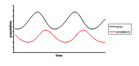
Solution to the equation: The solutions to the equations are periodic. The predator population follows the prey population.
Licenses & Attributions
CC licensed content, Shared previously
- Curation and Revision. Provided by: Boundless.com License: CC BY-SA: Attribution-ShareAlike.
CC licensed content, Specific attribution
- Differential equation. Provided by: Wikipedia Located at: https://en.wikipedia.org/wiki/Differential_equation. License: CC BY-SA: Attribution-ShareAlike.
- function. Provided by: Wiktionary Located at: https://en.wiktionary.org/wiki/function. License: CC BY-SA: Attribution-ShareAlike.
- derivative. Provided by: Wikipedia License: CC BY-SA: Attribution-ShareAlike.
- Differential equation. Provided by: Wikipedia License: CC BY-SA: Attribution-ShareAlike.
- Radioactive decay. Provided by: Wikipedia License: CC BY-SA: Attribution-ShareAlike.
- decay. Provided by: Wiktionary License: CC BY-SA: Attribution-ShareAlike.
- differential equation. Provided by: Wiktionary License: CC BY-SA: Attribution-ShareAlike.
- Differential equation. Provided by: Wikipedia License: CC BY: Attribution.
- Slope field. Provided by: Wikipedia License: CC BY-SA: Attribution-ShareAlike.
- Euler method. Provided by: Wikipedia License: CC BY-SA: Attribution-ShareAlike.
- normalize. Provided by: Wiktionary License: CC BY-SA: Attribution-ShareAlike.
- tangent. Provided by: Wiktionary License: CC BY-SA: Attribution-ShareAlike.
- differential equation. Provided by: Wiktionary License: CC BY-SA: Attribution-ShareAlike.
- Differential equation. Provided by: Wikipedia License: CC BY: Attribution.
- Slope field. Provided by: Wikipedia License: CC BY: Attribution.
- Euler method. Provided by: Wikipedia License: CC BY: Attribution.
- Separable partial differential equation. Provided by: Wikipedia License: CC BY-SA: Attribution-ShareAlike.
- fraction. Provided by: Wiktionary License: CC BY-SA: Attribution-ShareAlike.
- derivative. Provided by: Wikipedia License: CC BY-SA: Attribution-ShareAlike.
- differential equation. Provided by: Wiktionary License: CC BY-SA: Attribution-ShareAlike.
- Differential equation. Provided by: Wikipedia License: CC BY: Attribution.
- Slope field. Provided by: Wikipedia License: CC BY: Attribution.
- Euler method. Provided by: Wikipedia License: CC BY: Attribution.
- Provided by: Wikimedia Located at: https://upload.wikimedia.org/wikipedia/commons/b/b0/Wave_packet_(dispersion).gif. License: CC BY-SA: Attribution-ShareAlike.
- Logistic function. Provided by: Wikipedia License: CC BY-SA: Attribution-ShareAlike.
- non-linear differential equation. Provided by: Wikipedia License: CC BY-SA: Attribution-ShareAlike.
- boundary condition. Provided by: Wikipedia License: CC BY-SA: Attribution-ShareAlike.
- derivative. Provided by: Wikipedia License: CC BY-SA: Attribution-ShareAlike.
- Differential equation. Provided by: Wikipedia License: CC BY: Attribution.
- Slope field. Provided by: Wikipedia License: CC BY: Attribution.
- Euler method. Provided by: Wikipedia License: CC BY: Attribution.
- Provided by: Wikimedia Located at: https://upload.wikimedia.org/wikipedia/commons/b/b0/Wave_packet_(dispersion).gif. License: CC BY-SA: Attribution-ShareAlike.
- Logistic function. Provided by: Wikipedia License: CC BY: Attribution.
- differential equation. Provided by: Wiktionary License: CC BY-SA: Attribution-ShareAlike.
- Linear differential equation. Provided by: Wikipedia License: CC BY-SA: Attribution-ShareAlike.
- Linear equations. Provided by: Wikipedia Located at: https://en.wikipedia.org/wiki/Linear_equations. License: CC BY-SA: Attribution-ShareAlike.
- simultaneous equations. Provided by: Wikipedia License: CC BY-SA: Attribution-ShareAlike.
- linear equation. Provided by: Wiktionary License: CC BY-SA: Attribution-ShareAlike.
- Differential equation. Provided by: Wikipedia License: CC BY: Attribution.
- Slope field. Provided by: Wikipedia License: CC BY: Attribution.
- Euler method. Provided by: Wikipedia License: CC BY: Attribution.
- Provided by: Wikimedia Located at: https://upload.wikimedia.org/wikipedia/commons/b/b0/Wave_packet_(dispersion).gif. License: CC BY-SA: Attribution-ShareAlike.
- Logistic function. Provided by: Wikipedia License: CC BY: Attribution.
- Linear equations. Provided by: Wikipedia License: CC BY: Attribution.
- Lotkau2013Volterra equation. Provided by: Wikipedia License: CC BY-SA: Attribution-ShareAlike.
- predator. Provided by: Wiktionary License: CC BY-SA: Attribution-ShareAlike.
- prey. Provided by: Wiktionary License: CC BY-SA: Attribution-ShareAlike.
- differential equation. Provided by: Wiktionary License: CC BY-SA: Attribution-ShareAlike.
- Differential equation. Provided by: Wikipedia License: CC BY: Attribution.
- Slope field. Provided by: Wikipedia License: CC BY: Attribution.
- Euler method. Provided by: Wikipedia License: CC BY: Attribution.
- Provided by: Wikimedia License: CC BY-SA: Attribution-ShareAlike.
- Logistic function. Provided by: Wikipedia License: CC BY: Attribution.
- Linear equations. Provided by: Wikipedia License: CC BY: Attribution.
- Lotkau2013Volterra equation. Provided by: Wikipedia License: CC BY: Attribution.
